Analysis of Price Stackelberg Duopoly Game with Bounded Rationality
Abstract
The classical Stackelberg game is extended to boundedly rational price Stackelberg game, and the dynamic duopoly game model is described in detail. By using the theory of bifurcation of dynamical systems, the existence and stability of the equilibrium points of this model are studied. And some comparisons with Bertrand game with bounded rationality are also performed. Stable region, bifurcation diagram, The Largest Lyapunov exponent, strange attractor, and sensitive dependence on initial conditions are used to show complex dynamic behavior. The results of theoretical and numerical analysis show that the stability of the price Stackelberg duopoly game with boundedly rational players is only relevant to the speed of price adjustment of the leader and not relevant to the follower’s. This is different from the classical Cournot and Bertrand duopoly game with bounded rationality. And the speed of price adjustment of the boundedly rational leader has a destabilizing effect on this model.
1. Introduction
In the oligopolistic market, oligopoly firms compete in quantity or price. We all know that Cournot model [1] is one of the most famous quantity game models, in which all firms (players) are provided with naive expectations. Presently, boundedly rational quantity oligopoly game has been studied widely, and a player can choose his expectation rule from three different expectations: naive, bounded rational, and adaptive [2, 3]. Many duopoly quantity games with homogeneous or heterogeneous players have been studied under linear or nonlinear demand function and linear or nonlinear cost functions [2–7]. Similarly, some researchers have studied all sorts of triopoly quantity game models [8–13]. These studies find that there are some complex dynamic behaviors such as bifurcation and chaos in the oligopoly quantity game model.
Compared with quantity competition, maybe price competition is more general in a real market. One of the most classical price game models is the Bertrand model [14]. In Bertrand model, each firm will try to reduce its product price, until its products are selling at no profit. This result is called Bertrand paradox. However, the Bertrand paradox rarely appears in practice. One of the reasons is that completely homogeneous product is almost nonexistent. So, one way of avoiding the paradox is to allow the firms to sell differentiated products [15]. Similar to quantity competition, boundedly rational duopoly and triopoly price game models with differentiated products have been studied in [16–19].
In the above mentioned quantity and price game models, the one-short games are static; that is, each of the players in the game determines their quantity or price at the same time. However, dynamic game or sequential game is very common in the real market. We all know that the most classical sequential game is Stackelberg game [20, 21] in which one firm, the leader, commits to a strategy first and publicly, and then the remaining firms, the followers, observe the leader’s choice and make their decisions. The original Stackelberg game model is a quantity game with homogeneous product. Later, it was extended to the differentiated products for both quantity and price game. Vives [22] summarized the literature about the Stackelberg game model and pointed out that the relevant literature took the quantity for decision variable mostly. Until now there is little literature on price Stackelberg game. Consequently, there is no result for boundedly rational price Stackelberg in a differentiated products market. And its dynamic has not been studied. This paper aims to fill this gap.
This paper is organized as follows. In Section 2, the price Stackelberg duopoly game model with boundedly rational players is briefly described. The local stability condition of the equilibrium point is discussed in Section 3. In Section 4, numerical simulations are used to demonstrate the complex dynamics of our model. Finally, the conclusion of this paper is provided in Section 5.
2. The Model
In this work, the two firms (leader and follower) are boundedly rational players. They have no complete information of market, and they determine the price of production with the information of local profit maximization.
One can see that the form of this dynamical system is so different from the previous classical Cournot and Bertrand duopoly game with bounded rationality. And the product price of the leader at period n + 1 is only relevant to its own price of period n; but the product price of the follower at period n + 1 is determined by its own price of period n and the leader’s price of period n + 1. In addition, this model is unsymmetrical and this is different from the Zhang’s [16] and Peng’s model, [19], in which their models are symmetrical. Maybe these will give rise to different result and complicated dynamics from the boundedly rational Cournot and Bertrand duopoly game.
3. Equilibrium Points and Local Stability
Theorem 1. The boundary equilibrium point E1 of the system (15) is unstable.
Proof. The Jacobian matrix at E1 takes the form:
Next, we will investigate the local stability of the Nash equilibrium point E*.
3.1. Local Stability of Nash Equilibrium Point E*
So, we can state the following summarizing result.
Theorem 2. The Nash equilibrium E* of the dynamical system (15) is locally asymptotically stable provided that
These inferences will be demonstrated in Section 4.
4. Numerical Simulations
In order to be more clear and intuitive in understanding the complex dynamic behavior of the discrete dynamical system (15), numerical analysis is used to describe the dynamical evolution process. For convenience, we take a = 2, b = 0.5, c1 = 0.2, c2 = 0.4, d = 0.3 to study the local stability properties of the Nash equilibrium point. By calculation, we get the Nash equilibrium E* = (3.3439, 3.2032).
Figure 1 shows the price bifurcation diagram with respect to α1 (the adjustment speed of boundedly rational leader) of dynamical system (15) when α2 = 0.5. One can see the Nash equilibrium E* = (3.3439, 3.2032) is locally stable when the parameter α1 is small. As α1 increases, the Nash equilibrium point becomes unstable; that is, Period-2 and period-4 bifurcations appear and finally chaotic scenario occur. Definitely, when α1 > 0.7294, flip (period-doubling) bifurcation occurs and complex dynamic behavior begins to appear. Obviously, this fluctuation of system is harmful to both firms. One can conclude that the speed of adjustment of the boundedly rational leader α1 has a destabilizing effect to the dynamical system (15). The Largest Lyapunov exponent which corresponds to Figure 1 is plotted in Figure 2. This diagram also shows the relationship between the local stability of the Nash equilibrium point and the speed of adjustment of the boundedly rational leader α1. And one can obtain a better understanding of dynamical behaviors of the system (15).
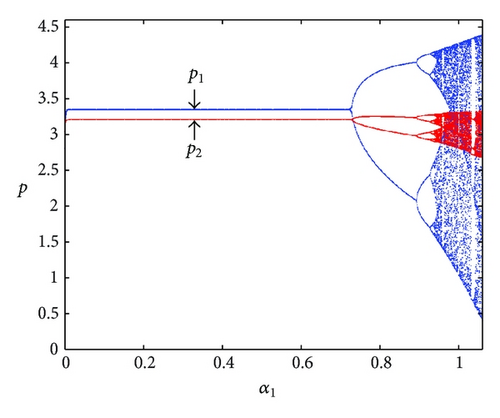
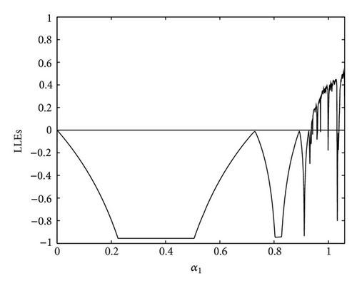
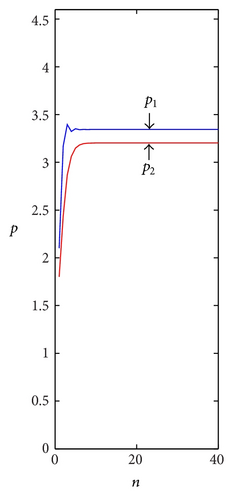
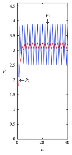
Figure 3 shows the price evolution with time when the dynamical system (15) is in the stable (α1 = 0.5), period-doubling bifurcations (α1 = 0.8), and chaotic state α1 = 1.0. As can be seen from Figure 3(a), along with the continuation of competitive cycle, the price of two firms will be stable in equilibrium state gradually after a series of fluctuation. And the price evolves into 2-period orbit gradually in Figure 3(b). But in Figure 3(c), the price is in chaos and takes on unordered change.
We draw the two-dimension flip bifurcation diagram in the parameters α1 and a (Figure 4(a)) and α1 and c1 (Figure 4(b)). In Figure 4, the Nash equilibrium is stable when the parameters α1, a, and c1are in the cyan-shaped area (stability region) and loses its stability with increasing value of α1. And the two-flip bifurcation cures are inverse function cures. This demonstrates what was mentioned above that stability region of the Nash equilibrium point is a decreasing function with respect to the market capacity a and the marginal cost c1.
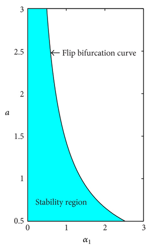
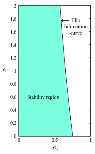
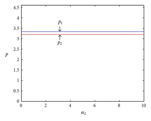
Figure 5 shows the price evolution process with respect to α2 (the speed of adjustment of the boundedly rational follower) of dynamical system (15) when α1 = 0.5. In Figure 4, the price is unalterable all the while and the dynamical system (15) is always locally stable. And this also demonstrates that the speed of adjustment of the boundedly rational follower has no effect on the game model.
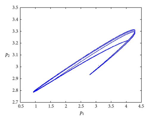
Strange attractor is one of the main features of chaotic motion. It exhibits fractal structure. Figure 6 shows the strange attractor in the phase plane (q1, q2) for the parameter values a = 2, b = 0.5, c1 = 0.2, c2 = 0.4, α1 = 1.07, and α2 = 0.5.
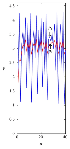
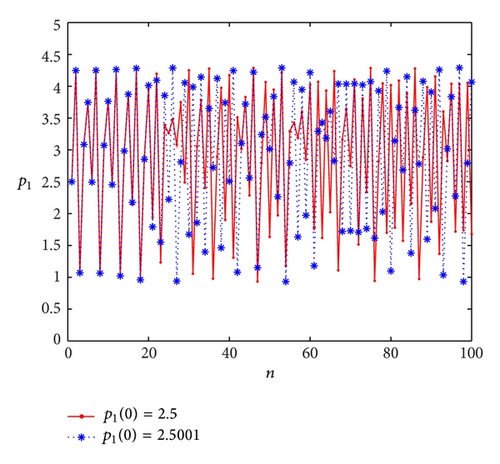
Sensitive dependence on initial conditions is another main characteristic of chaotic system. In order to demonstrate sensitive dependence on initial conditions of system (10), we simulate two orbits in Figure 7 for the parameter values a = 2, b = 0.5, c1 = 0.2, c2 = 0.4, α1 = 1.01, and α2 = 0.5. The red and blue curves start from the initial points (p1(0), p2(0)) = (2.5, 2.3) and (p1(0), p2(0)) = (2.5001,2.3), respectively. It shows that, at the beginning, they are indistinguishable, but after a number of iterations, the difference between them builds up rapidly.
5. Conclusion
In this paper we have proposed a price Stackelberg duopoly game model with boundedly rational players. The complex dynamical behaviors have been studied. In Nash equilibrium, the price of the leader is less than the follower’s and also less than equilibrium price of Bertrand game under the same assumption. The theoretical and numerical analysis shows the result that the stability of the dynamical system (15) is only relevant to the speed of price adjustment of the boundedly rational leader and not relevant to the follower’s. Definitely, the speed of price adjustment of the boundedly rational leader has a destabilizing effect and the follower’s has no effect on the dynamical system. This is different from the classical Cournot and Bertrand duopoly game with bounded rationality. Perhaps the reason of this is the Stackelberg-type game structure. The other type of price Stackelberg game, such as with heterogeneous player or different competition strategies, will be studied in future work.
Conflict of Interests
The authors declare that there is no conflict of interests regarding the publication of this paper.
Acknowledgments
The authors would like to thank the anonymous referees very much for their valuable comments and suggestions. This work was supported by Major Program of National Natural Science Foundation of China (71390521 and 71390523) and by National Natural Science Foundation of China (71101067, 71271103, 71301062, and 71301070).


