This paper investigates the freight empty cars allocation problem in railway networks with dynamic demands, in which the storage cost, unit transportation cost, and demand in each stage are taken into consideration. Under the constraints of capacity and demand, a stage-based optimization model for allocating freight empty cars in railway networks is formulated. The objective of this model is to minimize the total cost incurred by transferring and storing empty cars in different stages. Moreover, a genetic algorithm is designed to obtain the optimal empty cars distribution strategies in railway networks. Finally, numerical experiments are given to show the effectiveness of the proposed model and algorithm.

1. Introduction

Freight empty cars allocation aims to distribute the available empty cars from origins to destinations in the railway networks so that the demands can be satisfied with the minimized shipment costs. Since the railway freight transportation plays an important role in modern society, reasonable allocation of the empty cars with systematic optimization is actually a crucial issue for the railway companies. In recent decades, a lot of researchers have investigated freight empty cars allocation problem and presented a variety of models and algorithms. In literature, Misra [1] firstly proposed this problem in 1972 and set up a simple freight empty train allocation model in a time period with the minimum cost consumption. Transportation algorithm and simplex method were also designed to search for the optimal solution of the proposed model. Grain and Sinay [2] figured out the freight empty car allocation problem by a linear programming model, in which the objective was to arrange car flow assignment to satisfy the maximum proceeds. They adopted transportation algorithm and simplex method for the solutions of this model. Haghani [3] converted the freight empty car allocation problem into an inventory problem in cargo operation stations in order to allocate the freight cars in these stations. Kikuchi [4] structured the problem as a transshipment problem under the concept that a fleet of single-purpose freight cars were pooled at many loading points and emptied at unloading terminals in order to reduce empty car miles and time. Liu [5] firstly applied the computer technology to solve the freight empty car allocation problem, which provided technical guidance for the future study. Moreover, Xiong et al. [6] propounded an effective genetic algorithm to solve the large-scale network empty cars allocation problem and designed an adapted matrix coding mode, crossover operator, and mutation operator to improve the searching performance of the genetic algorithm.

Besides the above mentioned researches, recent studies always formulated this problem based on the standard transportation problem and traffic flow problem. As for the transportation problem based methods, Liu [7] investigated both the balanced transportation model and the unbalanced transportation model for the problem, which were solved by minimum element methods. X. Zhang and Q. Zhang [8] considered the problem based on the balanced transportation problem with the influence of the constraint conditions. Liang et al. [9] presented the concepts of alternative vehicles in unbalanced transportation model and constructed an optimization model with maximized profit. Lei et al. [10] introduced a stochastic programming model with probability chance-constraints and designed an efficient genetic algorithm to seek an approximate optimal solution. Narisetty et al. [11] proposed an optimization model for the empty car assignment problem based on the customer demand, which was implemented at Union Pacific Railroad to assign empty freight cars. The proposed approaches can further reduce transportation costs and improve delivery rate efficiency and customer satisfaction.

More recently, some researchers developed network flow models and optimization methods which could be regarded as references for the freight empty car allocation problem. For instance, Wang et al. [12] considered freight empty car allocation problem on the basis of quantity distribution and network matching flow and then designed ant colony algorithm to solve the proposed model. Laporte et al. [13] applied a game theoretic framework to research the railway transit network design problem. Dorfman and Medanic [14] developed a discrete event model for the feedback travel advance strategy, which can quickly handle perturbations in the schedule. Erkut and Gzara [15] applied the network flow strategy to hazardous material transportation and proposed a heuristic solution method to search a stable solution. In a large-scale railway network, Guo et al. [16] proposed the methods to merge the traffic flow in the main support stations and reduce nodes in railway networks, which can improve the efficiency of operations.

To understand the contributions of this research clearly, the detailed features will be summarized in Table 1 in comparison with some related works.

Table 1. The detailed features of different studies.

	Misra [1]	Kikuchi [4]	Lei et al. [10]	Joborn et al. [17]	This Paper
Problem description	A simple transportation problem	A transshipment problem	A balanced transportation problem	A network flow problem	A time-stage network flow problem
Formulation	A linear programming model	An improved linear programming model	A stochastic programming model	A capacitated network design model	A dynamic network flow model
Network	Physical network	Physical network	Physical network	Time-space network	Time-space network
Characteristics	—	Single-stage demand	Single-stage demand	Single-stage demand	Multi-stage demand
Algorithm	The simplex method	—	GA (genetic algorithm)	TS (tabu search)	GA (genetic algorithm)

It is easy to see in the literature that the majority of researches investigate this problem in certain environments, in which all the parameters are assumed to be static. In practice, since railway traffic is a complicated system, the demands of empty freight cars are always dynamic in most circumstances. To clearly state this characteristic, in this study, we particularly treat the demand at each destination as a stage-based demand, in which one stage corresponds to a prespecified time period. Then, we formulate the problem as a mathematical optimization model with multistage demands. Also, a genetic algorithm is particularly designed for the problem to efficiently generate the approximate optimal solution of the model.

The rest of this paper is organized as follows. In Section 2, an optimization model for freight empty cars allocation in railway networks and some preliminaries are presented. In Section 3, a genetic algorithm is designed to find an optimal solution for freight empty cars allocation problem. Some instances are given to show the effectiveness of the model and algorithm in Section 4. Conclusions are finally made in Section 5.

2. Formulation of the Problem

2.1. Problem Statement

Allocating empty cars is an important operation for railway companies to guarantee the normal operations of transportation activity. In traditional operation modes, empty cars are in general required to be transferred to the destination according to the prespecified demand that is always treated as a fixed quantity. However, due to the uncertainty of decision environments, the demand of freight empty cars at the destination is always changeable in the real-world applications (namely, the needs vary in different time periods). Thus, the traditional model will potentially cause a large number of empty backlogs or supply shortage, leading to the transportation task being unable to be accomplished effectively. Aiming to provide a framework for practical decisions, in this research we are particularly interested in the formulation of the model with dynamic demands and effective algorithms for the freight empty cars allocation problem.

In dynamic case, the time horizon will be divided into a variety of time periods, denoted by stages. Then, some important parameters in the problem will be reconsidered as the stage-based quantities, including the demand, cost, capacity, and so forth. For different stages, all of these parameters can be different according to the practical requirements, while they are assumed to be fixed quantities within each given stage. To formulate the dynamic empty cars allocation problem, we need to specify the following three types of constraints. (1) The first constraint concerns the traffic flow volume from supply stations, which is determined by the predicted demands in organization plans and train schedules. In particular, the traffic flow volume is required to be consistent with the supply capacity of each supply station. (2) The second constraint refers to the transportation capacities of stations and railway links. The total traffic flow on these stations and links cannot exceed the corresponding capacities. (3) The last constraint is associated with the demand of traffic flow volume. That is, all the dynamic demands need to be satisfied in each stage.

To clearly state the considered problem, we shall give an illustration in Figure 1, where stations 1 and 2, respectively, represent the supply station and demand station in the railway network. We here consider the following scenarios: in day 1, the demand of the destination is 20 empty cars, while the demand is 30 empty cars in day 2. Without considering stage-based demands, a total of 50 empty cars will be delivered to station 2 in day 1, leading to the waste of resources and the storage cost for unoccupied cars. On the other hand, if the demand is divided into two stages associated with different days, that is, D₁ = 20 and D₂ = 30, then the extra cost can be avoided if we allocate the empty cars according to the stage-based demands.

Details are in the caption following the image — **Figure 1**
Open in figure viewer PowerPoint

An illustration of delivery plans.

Hereinafter, some assumptions will be given in order to formulate the mathematical model.

(A1)
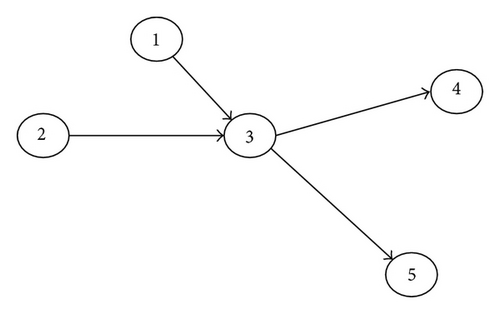
In order to characterize the considered railway network, an abstract graph, denoted by G(N, A), will be extracted from the physical network (see an illustration in Figure 2), in which N denotes the set of nodes representing the railway stations, and A is the set of directed links between adjacent nodes. Corresponding to the different stages, stage-based transportation cost will be treated as the weight of each link. Directed links indicate the transportation direction between two nodes.
(A2)
The demand, storage cost, and unit transportation cost in the considered time horizon are all dynamic, while these parameters in each stage are treated as constants.
(A3)
In the railway network, the total supply capacity in original stations is supposed to be greater than the total demand in destinations to guarantee the transportation activities.
(A4)
The demand in each stage should be satisfied. Unused empty cars can be left for the next stage with an extra storage cost.

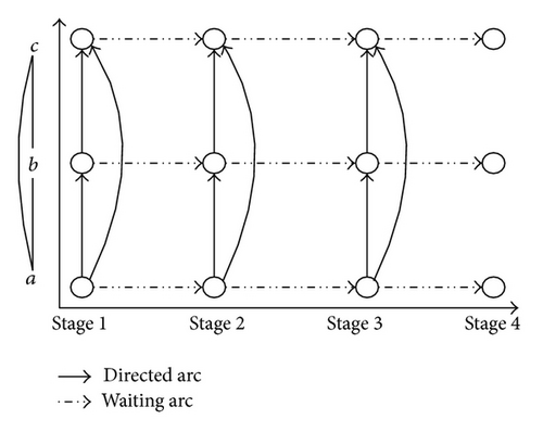
Here, to explicitly demonstrate the empty cars allocation process, an illustrative network, which consists of three node and three links, is given in Figure 3. To show the dynamics in the network, the time horizon is firstly divided into four stages. Then the right side of Figure 3 depicts the space-time network for the empty car allocating process, where each node represents the state of a physical node in each stage (for more detailed description for space-time networks, interested readers may refer to Yang and Zhou [18], Yang et al. [19]). Suppose that nodes a and c, respectively, denote the supply station and demand station. Then, two paths can be employed for the operations, that is, a → b → c and a → c, as shown in the arrow links. In the first stage, there will be some empty cars required to be transferred to station c from station a. If the transferred cars just satisfy the demand at station c, no storage cost occurs. Otherwise, if the number of transferred cars is greater than the demand at station c, then the unused empty cars should be delayed at this station, leading to an extra storage cost. The dotted arrow links in Figure 3 represent the waiting arcs for the unused empty cars at station c. Likewise, in the following stages, it is required that the summation of transferred cars and stored cars of the previous stages should also satisfy the stage-based demands. Then, in the process of allocating empty cars, the total cost can be separated into two parts: the transportation cost and storage cost. The aim is to generate the optimal allocation strategies in railway networks.

2.2. Mathematical Model

In this section, we shall formulate the freight empty cars allocation problem with dynamic demands as a stage-based network flow problem below.

2.2.1. Parameters and Notations

To formulate the mathematical model for this problem, some relevant parameters are firstly listed in Table 2.

Table 2. Parameters used in formulation.

Parameters	Definition
A	The set of links;
N	The set of nodes;
i, j	The index of nodes;
(i, j)	The index of link from node i to node j;
\|A\|	The total number of links;
\|N\|	The total number of nodes;
k	The different stages, k = 1,2, …, K;
	The unit transportation cost on link (i, j) in stage k;
o_s	Origin station which supplies empty cars, s = 1,2, …, S;
R_s	The supply amount of empty cars in station o_s;
d_t	Destination station which requires empty trains, t = 1,2, …, T;
D_t	The total demand of empty cars in station d_t;
Q_ij	The link capacity on link (i, j);
G_i	The turnover capacity at station i;
e_k	The unit storage cost for stage k;
	The demand of empty cars at station d_t for stage k.

2.2.2. Decision Variables

In this problem, the purpose is to generate an optimal transportation plan over the entire time horizon. As the multistage strategy will be considered, the decision variable can be treated as the amount of empty car flow corresponding to each link and stage. Then, we have the decision variable as

: denotes the number of empty cars delivered on link (i, j) for stage k, satisfying , where Z⁺ denotes the set of positive integers.

With this variable, the freight empty car allocation problem can be essentially treated as a traffic flow assignment process with the following constraint conditions.

2.2.3. System Constraints

To guarantee the feasibility of the allocation plans, we need to consider some system constraints in the process of allocating empty cars. Specifically, there are six types of system constraints in this model, which are presented as follows.

(i) The Supply Capacity Constraint. The available empty cars in supply station o_s should be more than or equal to the cars that are dispatched from this station o_s. We then have the following constraint:

(1)

(ii) The Demand Constraint. When the flow is delivered at the station d_t, it is required that the delivered flow volume

should meet the total demand D_t, which can be represented as

(2)

(iii) The Flow Balance Constraint. To keep the balance of the total flow, it is required that the amount of the inflow cars should be equal to the outflow cars at each station. We then have

(3)

(iv) The Link Capacity Constraint. In general, the transportation capacity on each link is not finite. To show this characteristic in the formulation, we particularly consider the link capacity constraint. That is, for each link (i, j), the flow volume cannot exceed the transportation capacity Q_ij, which can be represented as

(4)

(v) The Turnover Capacity Constraint. According to the real-world applications, a turnover capacity constraint should also be considered at each station. Then, at a transfer station i, the volume of traffic flow cannot exceed the turnover capacity G_i. The constraint can be represented as follows:

(5)

(vi) The Stage-Based Demand Constraint. As the total demand is separated as stage-based demand, the flow volume delivered to each destination and its stored empty cars should satisfy the demand

at station d_t for each stage; namely, if k = 1, there will be one constraint:

(6)

And if k = 2, the constraints should be

(7)

Considering all the stages, we formulate these constraints as follows:

(8)

With the stage-based demand constraint, we can ensure that the demand can be satisfied in each stage. When n = K, it is easy to see that (8) is the same to (2). Then, in the following discussion, we will not explicitly consider (2).

2.2.4. Objective Function

This problem aims to find the optimal allocation strategies with the minimized cost. As addressed in the illustration, the total cost in essence consists of two parts, namely, delivery cost in the network and storage cost in destinations.

The delivery cost refers to the expenses in the process of delivering empty cars. Since in stage k, the flow volume on link (i, j) is denoted by

, considering all the stages and links, we finally formulate the total delivery cost f₁(X) below:

(9)

In this problem, the freight empty cars will be delivered in different stages, which produce the following two situations. (1) One is that the traffic flow volume just meets the demand. That is, the delivered total empty cars are equal to the number of cars required in this stage. Then, no storage cost will be produced in this case. (2) The other one is that the number of empty cars is larger than that required in this stage. For this case, the redundant cars will be used in the next stage, resulting in the extra storage cost, which can be formulated as

(10)

So the total storage cost at destination d_t can be summarized as the following form:

(11)

Considering all the destinations, we finally formulate the total storage cost as

(12)

Then, the total cost for these two parts is

(13)

2.2.5. Mathematical Model

Consider the objective and constraints, the mathematical model of this problem can be formulated as follows:

(14)

In this model, the objective is to minimize the total cost in the railway transportation system. The first two constraints guarantee the rationality of the transportation activities. The third and fourth constraints ensure that the amount of traffic flow volume cannot exceed the capacities of each link and each node, respectively. The fifth constraint ensures that the stage-based demand can be satisfied with the demand constraints.

2.3. Model Analysis

To discuss the complexity of the proposed formulation, the following discussion aims to analyze the characteristics of the proposed model. We firstly focus on the number of constraints in the model, which are displayed in Table 3.

Table 3. The amount of constraints in each constraint condition.

Constraints	Number
(1)	S
(3)	K · (\|N\| − S − T)
(4)	\|A\|
(5)	\|N\| − S − T
(8)	K · T

Total number	K · (\|N\| − S) + \|N\| + \|A\| − T

An illustration will be given in the following to demonstrate the complexity of the proposed model. Consider a network with 20 nodes and 50 links. In this network, suppose that there are three origin stations and three destination stations. A total of three stages will be taken into consideration. With the assumption above, since a total of 9 paths need to be considered, the number of decision variables should be 150 over the entire network. Moreover, a total of 118 constraints need to be included in the model.

Note that when the network scale increases, the number of constraints and variables will increase to a great extent accordingly, which potentially leads to the difficulties in calculation. Then, in order to simplify the computational complexity in the process of allocating cars, in the next section, we shall transform the arc-based solutions into route-based solutions, in which constraint (4) and constraint (5) can be merged into one constraint. Thus, it can decrease the complexity of the solution methods expectedly. The following section will design genetic algorithm to search for an approximate optimal solution.

3. Genetic Algorithm

In practice, it is rather difficult to solve the large-scale freight empty cars allocation problem efficiently. Because of this, we aim to design an approximation algorithm in this section, seeking a feasible solution which can replace the best solution approximatively.

The approximation algorithm is also called heuristic algorithms, which include tabu search algorithm, simulated annealing algorithm, genetic algorithm, neural network algorithm, and ant colony algorithm. As the genetic algorithm is a kind of direct searching method which does not depend on the specific characteristics of problems, it is efficient and effective in solving a variety of real-world problems. The principle of genetic algorithm is to simulate the mechanism of the living beings evolving and natural choosing. It was well developed by many researchers. Up to now, the genetic algorithm has been successfully used to solve practical optimization problems, such as transportation problem (Gen et al. [20]), machine scheduling problem (Vallada and Ruiz [21]), vehicle routing problem (Baker and Ayechew [22]), network optimization (Ukkusuri et al. [23]) and railway operation problem (Yang et al. [24, 25], Xu et al. [26]).

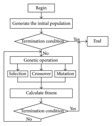
In general, the procedure of genetic algorithm is as follows: (1) randomly generate a certain number of chromosomes; (2) evaluate the quality of those chromosomes with fitness function according to some criteria; (3) obtain fine chromosomes via selection, crossover, and mutation operations. Figure 4 is the procedure of this algorithm.

3.1. Solution Representation

In solving the empty car allocation problem, we need firstly to determine the solution representation in the genetic algorithm. As described in the model, the solution is represented as link-based flow in each link. To simplify the complexity of computation, we here particularly introduce the path-based solution representation in the genetic algorithm. Since link-based flow can be finally split into the flow on different paths between different OD pairs (here, “OD pair” is an abbreviation for the origin and destination terminals), in this method, potential paths should be determined firstly, and then we determine the flow volume on each path to satisfy the demand of each destination.

An illustration is given to show the difference between link-based solution and path-based solution, depicted in Figure 5.

In Figure 5, each path consists of three nodes, namely, a supply station, an intermediate station and a demand station. Suppose that two-stage demands exist in this network. According to the link-based solution, there will be 4 variables and 8 constraints in total. If we set the variables and constraints in a path instead of in links, there will be only 2 variables and 5 constraints totally, both less than those in link-based representation. In reality, the scale of network structure will be more complex than this simple transportation network. So the number of decision variables with link-based representation is more than that with path-based representation. In order to reduce the algorithm complexity and obtain an approximate optimal solution, the following discussion particularly adopts the path-based solution representation.

In this procedure, a path, denoted by P, is represented by a sequence of ordered nodes. For instance, the set P = {1, 3, 5, 9} denotes the following path:

(15)

In genetic algorithm, all the potential paths should be generated between each OD pair, which serve as the transport paths in the process of delivering empty cars.

In the genetic algorithm, each population consists of pop_size feasible solutions as chromosomes. Since we use the path-based solution in the algorithm, each solution in population will be generated randomly. Moreover, for each generated solution, its feasibility will be checked by transforming it into link-based solution. If all the constraints can be satisfied, this solution is a feasible solution. Otherwise, the solution will be regenerated randomly. At the beginning of the algorithm, a total of pop_size solutions should be produced. In this paper, we set path-based decision variables as nonnegative integers, denoting the number of empty cars transferred on the corresponding path.

3.2. Selection Operation

In the genetic algorithm, the role of selection operation is to produce a new population for the following crossover and mutation operations. In the initial population, the chromosomes are first ranked from the good to the bad according to their objectives. Without loss of generality, the rearranged chromosomes are denoted by X₁, X₂, …, X_{pop_size}, where X₁ and X_{pop_size} denote the best and the worst chromosomes, respectively. The rank-based fitness of each chromosome can be calculated by the following formula:

(16)

where β ∈ (0,1) is a predetermined parameter.

Here, we give the detailed procedure to show the selection process below.

Step 1. Compute the fitness of each individual in population fitness(X_l), l = 1,2, …, pop_size.

Step 2. Compute the cumulative probability q_l of each individual in population. And q_l can be calculated by the following formula:

(17)

Step 3. Generate a random number r in (0,1).

Step 4. If r < q₁, select X₁. If q_l−1 < r ≤ q_l, then chromosome X_l will be selected as a member of the new population.

Step 5. Repeat Step 3 and Step 4 for pop_size times.

3.3. Crossover Operation

Crossover operations aim to generate a new population in the searching process. Before this operation, the parents should be specified according to the predetermined crossover probability P_c. To this end, the following procedure is designed.

Step 1. Let h = 1.

Step 2. Randomly generate a number r in the interval (0,1).

Step 3. If r < P_c, chromosome X_h is selected to take part in crossover operation; otherwise, X_h will not be selected.

Step 4. Let h + +, if h ≤ pop_size, go to Step 2.

Step 5. Record the selected chromosomes.

After the parent chromosomes are selected, any two chromosomes can be used for crossover operation. Suppose that the two parent chromosomes are X₁ and X₂ and the children chromosomes are and . The following process is designed to perform the crossover operation.

Step 1. Randomly generate a parameter α in interval (0,1), let and .

Step 2. Reset and as integer vectors by rounding operation for each element.

Step 3. Check the feasibility of the two children chromosomes and . If the children chromosomes are feasible, replace the parents chromosomes by them; Otherwise, remain the parents chromosomes.

Step 4. Record the new population.

3.4. Mutation Operation

In order to avoid premature convergence, the mutation operation is necessary in the searching process of genetic algorithm. Like the crossover operation, we firstly need to determine the chromosomes for mutation operations. The number of chromosomes selected to perform mutation operation is also completely based on the predetermined mutation probability P_m.

Step 1. Let h = 1.

Step 2. Randomly generate a number r in the interval (0,1).

Step 3. If r < P_m, chromosome X_h is selected to take part in mutation operation; otherwise, X_h is not the one.

Step 4. Let h + +. If h ≤ pop_size, go to Step 2.

Step 5. Record the selected chromosomes.

For each selected parent chromosome X_h, we are aiming to generate the children chromosome . The following procedure is designed to perform mutation operations.

Step 1. Randomly generate a mutation direction vector , in which all of the elements are generated in the interval (−1,1).

Step 2. Let , where m is a positive integer.

Step 3. Reset as an integer vector by rounding operation for each element.

Step 4. Check the feasibility. If is feasible, let replace X_h. Otherwise, set m = m/2, go to step 2.

3.5. Procedure of Algorithm

For the completeness of this paper, we shall give the detailed procedure of the algorithm in the following.

Step 1. Randomly generate pop_size chromosomes in the population.

Step 2. Perform the selection operation.

Step 3. Perform the crossover operation.

Step 4. Perform the mutation operation.

Step 5. Repeat Step 2 to Step 4 for a given number (denoted by Generation) of times.

Step 6. Output the best solution.

4. Model Test and Computational Results

In this section, we give two numerical examples with different scales to illustrate the effectiveness of the proposed methods, in which the experiments are implemented by using C++ software in a personal computer with Intel(R) Core(TM) i5-3317U 1.70 GHz.

4.1. Small-Scale Instance

In the first set of experiments, we consider a small-scale network, shown in Figure 2. This network consists of five nodes and four links, in which nodes 1 and 2 represent origin stations, node 3 denotes an intermediate station, and nodes 4 and 5 represent destination stations. In this network, it is easy to see that four potential paths exist between different OD pairs; that is, 1 → 3 → 4, 1 → 3 → 5, 2 → 3 → 4, 2 → 3 → 5.

In this network, we consider two-stage based demands. The detailed data are given as link 1 → 3: (3,3, 65), link 3 → 4: (2,5, 80), link 2 → 3: (2,2, 55), and link 3 → 5: (3,2, 40), where the numbers in brackets denote unit transportation cost for stage one, unit transportation cost for stage two, and transfer capacity of the link. Additionally, at transfer station 3, the turnover capacity is 150. In origin stations 1 and 2, the numbers of available cars are 110 and 60, respectively.

Besides, it is possible that the storage cost can occur in the allocation plan. Then, the unit storage cost for different stages are given in Table 4.

Table 4. Storage cost and demand in destination stations.

Station	Stage 1		Stage 2
Station	Storage cost	Demand	Storage cost	Demand
4	2	30	1	50
5	1	40	2	30

It is easy to see in this problem that there are a total of 8 variables and 13 constraints in the allocation process. As we formulate this problem as a linear programming model, we firstly use the Lingo software to calculate this problem, where the optimal objective turns out to be 830 and the optimal solution is given in Table 5.

Table 5. The best solution solved by Lingo software.

Variable
Value	65	25	55	5	80	0	40	30

In the following, we shall investigate the performance of the genetic algorithm. To this end, we particularly list the best solutions encountered during the first 16 generations to analyze the convergence of the algorithm, shown in Table 6.

Table 6. The best solutions and objective values in different generations.

Generation									Value
1	44	56	44	8	47	33	41	31	883
2	40	58	45	8	45	35	40	31	877
3	40	58	45	7	45	35	40	30	873
4	42	54	45	9	47	33	40	30	869
5	52	42	39	18	51	29	40	29	867
6	42	52	46	10	48	32	40	30	866
7	49	49	46	6	55	25	40	30	863
8	52	45	53	0	63	17	42	28	858
9	52	44	54	0	64	16	42	28	856
10	50	44	56	0	65	15	41	29	851
11	52	40	56	2	66	14	42	28	850
12	52	40	57	1	67	13	42	28	849
13	47	44	58	1	65	15	40	30	846
14	46	44	59	1	65	15	40	30	845
15	47	43	60	0	65	15	40	30	843
16	48	42	60	0	65	15	40	30	842

In Table 6, it is easy to see that all decision variables can approach the best solution gradually in the searching process, and the approximate optimal objective can be quickly achieved in a short time. To further show the convergence process of the solution, Figure 6 gives the detailed variation of decision variables and in the first 16 iterations.

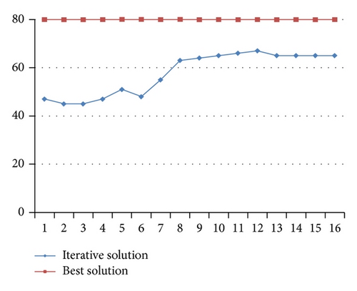
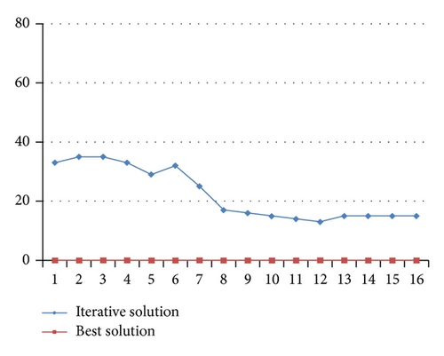
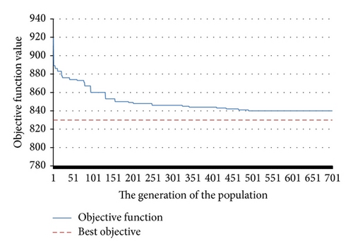
It follows from Figure 6 that, for decision variables and , they can approach to their optimal values (obtained by Lingo software) quickly with a relative small undulation, and this tendency is almost kept in the following generations. Additionally, the encountered optimal objective will maintain 840 (see Figure 7) after about 500 generation, with +10 error to the best objective obtained by Lingo software, leading to a relative small error 1.2%, which shows the effectiveness of genetic algorithm for solving this problem.

4.2. A Large-Scale Instance in China

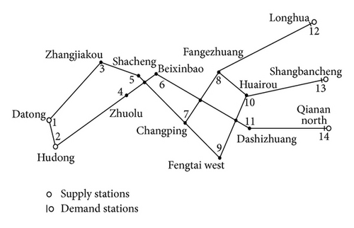
In the following, we propose a computational experiment derived from real-life instances of the railway network in Beijing, Hebei, and Shanxi province of China. In this instance, a total of 103 stations are located on the network. In particular, we omit some intermediate points for displaying convenience in Figure 8, where some important terminal stations are indexed by numbers, corresponding to their positions in the real-life network. In this network, a path can be represented by a sequence of terminal stations. Figure 9 gives an illustration for a path from station 1 to station 12, denoted by 1 → 3 → 5 → 6 → 8 → 12. In the real case, there still exist a total of 47 intermediate stations on this path (besides origins and destinations). In this set of experiments, suppose that there are two origins (node 1 and node 2) and three destinations (node 12, node 13, and node 14). We use the path-based solution for the empty car allocation process. Then, we first determine eleven potential paths for the solution process, listed in Table 7. Furthermore, the unit transportation cost is also given for different links. For instance, the first path consists of five links, then (3, 2, 1, 2, 4) represents the corresponding unit transportation cost on each link (here, we adopt invariant link unit transportation cost over different stages).

Table 7. The considered paths and unit transportation cost on arcs.

Number	OD	Paths	Unit cost on arcs
1	1 → 12	1 → 3 → 5 → 6 → 8 → 12	(3,2, 1,2, 4)
2	1 → 12	1 → 3 → 5 → 7 → 8 → 12	(3,2, 3,2, 4)
3	1 → 13	1 → 3 → 5 → 7 → 8 → 10 → 13	(3,2, 3,2, 1,3)
4	1 → 13	1 → 3 → 5 → 7 → 9 → 10 → 13	(3,2, 3,1, 2,3)
5	1 → 14	1 → 3 → 5 → 6 → 11 → 14	(3,2, 1,1, 2)
6	2 → 12	2 → 4 → 6 → 8 → 12	(2,1, 2,4)
7	2 → 12	2 → 4 → 7 → 8 → 12	(2,2, 2,4)
8	2 → 13	2 → 4 → 6 → 8 → 10 → 13	(2,1, 2,1, 3)
9	2 → 13	2 → 4 → 7 → 8 → 10 → 13	(2,2, 2,1, 3)
10	2 → 13	2 → 4 → 7 → 9 → 10 → 13	(2,2, 1,2, 3)
11	2 → 14	2 → 4 → 6 → 11 → 14	(2,1, 1,2)

In addition, we assume that supply capacities at stations 1 and 2 are 275 and 240, respectively. The empty cars allocating process are divided into three stages, and stage-based demands and storage costs are listed in Table 8, respectively.

Table 8. The demand and unit storage cost in different stages.

Stage	Time period	Node 12	Node 13	Node 14	Storage cost
1	8:00~16:00	75	50	40	7
2	16:00~24:00	90	85	50	4
3	24:00~8:00	35	20	30	1

This set of experiment is implemented by genetic algorithm in C++ software on a personal computer. To test the robustness of the proposed algorithm, we perform ten experiments with different parameters in the genetic algorithm. The results are given in Table 9 for analysis convenience.

Table 9. The comparison of the optimal objectives.

	Pop_size	P_c	P_m	Generation	Objective value	Error (%)
1	10	0.4	0.4	1000	5062	1.52
2	20	0.4	0.4	1000	5036	1.01
3	20	0.6	0.4	1000	5036	1.01
4	20	0.6	0.4	5000	5022	0.74
5	30	0.6	0.4	1000	5010	0.50
6	20	0.6	0.8	1000	5026	0.82
7	20	0.6	0.8	5000	4994	0.18
8	30	0.8	0.4	1000	5010	0.50
9	30	0.6	0.8	2000	4985	0
10	30	0.6	0.8	5000	4985	0

Average value						0.628
Variance						0.0022

As shown in Table 9, by using different parameters, we can produce different approximation optimal solutions and objectives. When setting pop_size = 30, P_c = 0.6, and P_m = 0.8, we finally produce the best objective 4985. In addition, the relative errors are also computed to show the performance of the algorithm, which can be calculated according to the following equation:

(18)

Obviously, for different experiments, the errors of objective values are not larger than 1.52%. In particular, the average error and error variance are only 0.628% and 0.0022%, respectively, which shows the steadiness of the algorithm.

To analyze the searching process of the proposed algorithm, we especially consider the computational results with parameters P_c = 0.6 and P_m = 0.8. Moreover, three experiments with pop_size = 15, 20, and 30, respectively, are implemented. Figure 10 gives the convergence of the optimal objectives with respect to different experiments.

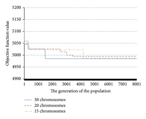
It is easy to see from this figure that, with different scales of population, the approximate optimal solution can be quickly achieved almost within 4000 generations. As expected, when we set a larger population, the optimal solution can be obtained with less generation in the searching process.

Finally, we give a comparison with the single-stage model to further show the effectiveness of the proposed approaches in this study. Specifically, the sum of the stage-based demands given in Table 8 will be considered as the demand in the single-stage model, and storage cost will be omitted in the process of allocating empty cars. Under this consideration, the best objective value for allocating empty cars turns out to be 7130 by using Lingo optimization software, which enhances the total transportation cost by 30% compared with the stage-based model.

5. Conclusions

This paper investigated a railway freight empty car allocation problem in the dynamic decision-making environment, in which the stage-based demands are considered, and the cost is divided into transfer cost and storage cost at destinations. To characterize this problem mathematically, an integer linear programming model was formulated with the minimization of total involved cost based on the network flow optimization. To generate approximate optimal solutions, a genetic algorithm with path-based solution representation is designed to seek the optimal empty car distribution strategies in railway networks. The numerical experiments are executed to show the performance of the proposed approaches. In particular, compared to the single-stage model, the total transportation cost in our model can be reduced by almost 30%, which implies the effectiveness of the proposed approaches.

The future research can be focused on the following two aspects. (1) The model can be generalized to the uncertainty environments within the framework of uncertain programming methods, since the real-life decision systems for railway operations are essentially in the state of uncertainty (see Yang et al. [19, 25] and Li et al. [27]). (2) More exact algorithms can be expectedly developed to further enhance the quality of the generated solutions.

Conflict of Interests

The authors declare that there is no conflict of interests regarding the publication of this paper.

Acknowledgments

This research was supported by the National Natural Science Foundation of China (no. 71271020), Research Foundation of State Key Laboratory of Rail Traffic Control and Safety, Beijing Jiaotong University (no. RCS2014ZT02), the National Basic Research Program of China (no. 2012CB725400), and the Beijing Natural Science Foundation (no. 9144031).

References

1 Misra S. C., Linear programming of empty wagon disposition, Rail International. (1972) 3, no. 3, 151–158, 2-s2.0-0015301034.
Google Scholar
2 Grain M. T. F. and Sinay M. C. F. D., Optimal distribution of empty railroad cars, Proceedings of the 1st International Congress in France of Industrial Engineering and Management, 1986, Ecole Centrale de Paris, France, 21–26.
Google Scholar
3 Haghani A. E., Rail freight transportation: a review of recent optimization models for train routing and empty car distribution, Journal of Advanced Transportation. (1987) 21, no. 2, 147–172, https://doi.org/10.1002/atr.5670210205, 2-s2.0-0023360630.
10.1002/atr.5670210205
Google Scholar
4 Kikuchi S., Empty freight car dispatching model under freight car pool concept, Transportation Research Part B. (1985) 19, no. 3, 169–185, 2-s2.0-0022267390.
10.1016/0191-2615(85)90001-3
Web of Science® Google Scholar
5 Liu M., The exploration of railway empty car allocating problem by using computer technology, Railway Transport and Economy. (1987) no. 6, 29–32.
Google Scholar
6 Xiong H., Lu W., and Wen H., Genetic algorithm used in railway empty car allocating problem, China Railway Science. (2002) 23, no. 4, 118–121.
Google Scholar
7 Liu H., The mathematical model in empty car adjustment technical planning, TMIS Engineering. (2002) 10, 29–31.
Google Scholar
8 Zhang X. and Zhang Q., Study on the optimization method of empty wagon distribution based on knowledge constraints, Journal of the China Railway Society. (2003) 25, no. 6, 14–20, 2-s2.0-0345768986.
CAS Google Scholar
9 Liang D., Lin B., Yan H., and Li J., Study of railway empty car distribution with substitution of empty car types, Journal of the China Railway Society. (2005) 27, no. 4, 1–5, 2-s2.0-24344467093.
Google Scholar
10 Lei Z., He S., Song R., and Cai J., Stochastic chance-constrained model and genetic algorithm for empty car distribution in railway transportation, Journal of the China Railway Society. (2005) 27, no. 5, 1–5, 2-s2.0-27744434678.
Google Scholar
11 Narisetty A. K., Richard J. P., Ramcharan D., Murphy D., Minks G., and Fuller J., An optimization model for empty freight car assignment at Union Pacific Railroad, Interfaces. (2008) 38, no. 2, 89–102, https://doi.org/10.1287/inte.1070.0330, 2-s2.0-61349118132.
10.1287/inte.1070.0330
Web of Science® Google Scholar
12 Wang D., Yan H., and Tan Y., Network node of railway refrigerator empty car adjustment in ant colony algorithm, China Railway Science. (2008) 29, no. 2, 131–135, 2-s2.0-42549135969.
Google Scholar
13 Laporte G., Mesa J. A., and Perea F., A game theoretic framework for the robust railway transit network design problem, Transportation Research Part B: Methodological. (2010) 44, no. 4, 447–459, https://doi.org/10.1016/j.trb.2009.08.004, 2-s2.0-77549085438.
10.1016/j.trb.2009.08.004
Web of Science® Google Scholar
14 Dorfman M. J. and Medanic J., Scheduling trains on a railway network using a discrete event model of railway traffic, Transportation Research Part B: Methodological. (2004) 38, no. 1, 81–98, https://doi.org/10.1016/S0191-2615(03)00006-7, 2-s2.0-0142156064.
10.1016/S0191-2615(03)00006-7
Web of Science® Google Scholar
15 Erkut E. and Gzara F., Solving the hazmat transport network design problem, Computers and Operations Research. (2008) 35, no. 7, 2234–2247, https://doi.org/10.1016/j.cor.2006.10.022, 2-s2.0-36348981523.
10.1016/j.cor.2006.10.022
Web of Science® Google Scholar
16 Guo P., Lin B., and Yu Y., Section center optimization method in large-scaled network car deployment, China Railway Science. (2001) 22, no. 2, 122–128.
Google Scholar
17 Joborn M., Crainic T. G., Gendreau M., Holmberg K., and Lundgren J. T., Economies of scale in empty freight car distribution in scheduled railways, Transportation Science. (2004) 38, no. 2, 121–134, https://doi.org/10.1287/trsc.1030.0061, 2-s2.0-3042666735.
10.1287/trsc.1030.0061
Web of Science® Google Scholar
18 Yang B. L. and Zhou X., Constraint reformulation and lagrangian relaxation-based solution algorithm for a least expected time path problem, Transportation Research B. (2014) 59, 22–44, https://doi.org/10.1016/j.trb.2013.10.012.
10.1016/j.trb.2013.10.012
CAS Web of Science® Google Scholar
19 Yang L., Zhou X., and Gao Z., Credibility-based rescheduling model in a double-track railway network: a fuzzy reliable optimization approach, Omega. (2014) 48, 75–93.
10.1016/j.omega.2013.11.004
Web of Science® Google Scholar
20 Yang B. L. and Zhou X., Constraint reformulation and lagrangian relaxation-based solution algorithm for a least expected time path problem, Transportation Research Part B. (2014) 59, 22–44.
10.1016/j.trb.2013.10.012
CAS Web of Science® Google Scholar
21 Vallada E. and Ruiz R., A genetic algorithm for the unrelated parallel machine scheduling problem with sequence dependent setup times, European Journal of Operational Research. (2011) 211, no. 3, 612–622, https://doi.org/10.1016/j.ejor.2011.01.011, MR2774437, 2-s2.0-79952187971.
10.1016/j.ejor.2011.01.011
Web of Science® Google Scholar
22 Baker B. M. and Ayechew M. A., A genetic algorithm for the vehicle routing problem, Computers & Operations Research. (2003) 30, no. 5, 787–800, https://doi.org/10.1016/S0305-0548(02)00051-5, 2-s2.0-0037395316.
10.1016/S0305-0548(02)00051-5
Web of Science® Google Scholar
23 Ukkusuri S. V., Mathew T. V., and Waller S. T., Robust transportation network design under demand uncertainty, Computer-Aided Civil and Infrastructure Engineering. (2007) 22, no. 1, 6–18, https://doi.org/10.1111/j.1467-8667.2006.00465.x, 2-s2.0-33750972613.
10.1111/j.1467-8667.2006.00465.x
Web of Science® Google Scholar
24 Yang L., Li K., Gao Z., and Li X., Optimizing trains movement on a railway network, Omega. (2012) 40, no. 5, 619–633, https://doi.org/10.1016/j.omega.2011.12.001, 2-s2.0-84855433912.
10.1016/j.omega.2011.12.001
Web of Science® Google Scholar
25 Yang L., Gao Z., and Li K., Railway freight transportation planning with mixed uncertainty of randomness and fuzziness, Applied Soft Computing Journal. (2011) 11, no. 1, 778–792, https://doi.org/10.1016/j.asoc.2009.12.039, 2-s2.0-77957914119.
10.1016/j.asoc.2009.12.039
Web of Science® Google Scholar
26 Xu X., Li K., Yang L., and Ye J., Balanced train timetabling on a single-line railway with optimized velocity, Applied Mathematical Modelling. (2014) 38, no. 3, 894–909, https://doi.org/10.1016/j.apm.2013.07.023, MR3160495, 2-s2.0-84880856693.
10.1016/j.apm.2013.07.023
Web of Science® Google Scholar
27 Li S., Yang L., Li K., and Gao Z., Robust sampled-data cruise control scheduling of high-speed train, Transportation Research Part C. (2014) 46, 274–283, https://doi.org/10.1016/j.trc.2014.06.004.
10.1016/j.trc.2014.06.004
Web of Science® Google Scholar

Citing Literature

All articles

Allocating Freight Empty Cars in Railway Networks with Dynamic Demands

Abstract

1. Introduction