This paper aims to enlarge the family of one-class classification-based control charts, referred to as OC-charts, and extend their applications. We propose a new OC-chart using the K-means data description (KMDD) algorithm, referred to as KM-chart. The proposed KM-chart gives the minimum closed spherical boundary around the in-control process data. It measures the distance between the center of KMDD-based sphere and the new incoming sample to be monitored. Any sample having a distance greater than the radius of KMDD-based sphere is considered as an out-of-control sample. Phase I and II analysis of KM-chart was evaluated through a real industrial application. In a comparative study based on the average run length (ARL) criterion, KM-chart was compared with the kernel-distance based control chart, referred to as K-chart, and the k-nearest neighbor data description-based control chart, referred to as KNN-chart. Results revealed that, in terms of ARL, KM-chart performed better than KNN-chart in detecting small shifts in mean vector. Furthermore, the paper provides the MATLAB code for KM-chart, developed by the authors.

1. Introduction

In recent years, several attempts have been proposed to integrate data mining with statistical process control (SPC) [1–6]. The objective was to overcome the limitations of traditional parametric control charts especially the normality assumption, which may not be applicable in the case of modern manufacturing systems. The most commonly applied data mining technique in SPC is one-class classification. Actually, one-class classification methods have been widely used for process monitoring [7–12]. The principle of one-class consists in constructing a sphere which contains the maximum of data with minimum volume. This sphere distinguishes in-control process data, also known as target data, from out-of-control process data. The shape and volume of the one-class depend on the used one-class classifier, also known as data description algorithm. The one-class approach was applied to develop a new family of control charts called one-class classification-based control charts, referred to as OC-charts.

Several types of one-class classifiers exist in the literature. For instance, only two one-class classifiers were used to develop control charts, named the support vector data description (SVDD) algorithm [13] and the k-nearest neighbor data description (KNNDD) algorithm [14]. Sun and Tsung [15] used SVDD to develop the kernel distance-based multivariate control chart, also known as the K-chart, which is considered as the first OC-chart that uses support vector principles. When monitoring more than two variables, the K-chart uses kernel methods that provide the advantage of dealing with high-dimension data. During the last decade, the K-chart has received significant attention and has witnessed several improvements through many works [16–19].

The SVDD algorithm was also employed to develop other control charts such as the SVDD based multivariate cumulative sum control chart [20], monitor batch process [21], monitor nonlinear processes [22], and perform industrial calibration [23]. Despite its successful application, the high computational cost of SVDD remains its main drawback. Actually, the SVDD algorithm loses its efficiency when the size of the training data becomes large. To overcome this shortcoming, Sukchotrat et al. [24] proposed the use of KNNDD algorithm to develop the KNN-chart. KNNDD is a simple and fast algorithm that performs better with high dimensional data and does not consume much time during the training phase. Gani and Limam [25] compared the performance of the K-chart and the KNN-chart and demonstrated that the K-chart is sensitive to small shifts in mean vector, while the KNN-chart is sensitive to moderate shifts in mean vector.

This paper investigates the use of another one-class classifier which is the K-means data description (KMDD) algorithm to construct a new OC-chart, referred to as the KM-chart. The objective of this work is twofold. First, we aim to enlarge the family of OC-charts and extend their applications by showing the methodology of their construction and providing the necessary software codes. Second, we attempt to propose an OC-chart that can compete with K-chart and KNN-chart in terms of the average run length (ARL) criterion.

The rest of this paper is organized as follows. A review of OC-charts is presented in Section 2. The proposed KM-chart is introduced in Section 3. Construction methodology of the KM-chart using a real data example is shown in Section 4, while performance analysis of the proposed control chart is discussed in Section 5. Section 6 summarizes this paper.

2. Background on OC-Charts

In the literature, there are two common OC-charts which are the K-chart and the KNN-chart. In the following, we give a review of these control charts.

2.1. The K-Chart

The K-chart relies on SVDD algorithm, which an unsupervised one-class classifier, to fit a sphere around the target data. This sphere is determined by solving the following quadratic programming

()

subject to

()

where F, a, and R, are, respectively, the cost function to minimize, the center and the radius of the sphere. Equation (2) shows that the vector of quality characteristics, denoted by x_i, having a distance smaller than the radius are considered as target. To allow the possibility of having outliers in the training set, the distance from x_i to the center a should not be strictly smaller than R², and larger distances should be penalized. Therefore, we introduce slack variables ξ_i ≥ 0 and the minimization problem becomes

()

subject to

()

where C > 0 is a parameter introduced for the trade-off between the volume of the sphere and the errors.

Equation (4) can be incorporated into (3) by using Lagrange multipliers

()

with the Lagrange multipliers α_i ≥ 0 and η_i ≥ 0, L should be minimized with respect to R, a, and ξ_i and maximized with respect to α_i and η_i. Setting partial derivatives of L, we obtain

()

From (8), α_i = C − η_i, α_i ≥ 0, and η_i ≥ 0, then Lagrange multipliers η_i can be removed and we have

()

By substituting (6) and (8) into (5), we have

()

subject to

()

A test sample, denoted by z, is accepted when its distance is smaller or equal to the radius. This is equivalent to

()

Generally, data is not spherically distributed. To make the method more flexible, the vectors of x_i are transformed to a higher dimensional feature space. The inner products in (10) and (12) are substituted by a kernel function K(x_i, x_j). In a higher dimension, the sphere becomes a complex form called “hypersphere.” The problem of finding the optimal hypersphere is given by

()

subject to (11).

A test sample z is accepted when

()

The construction of the K-chart consists in determining which samples are support vectors (SVs) by solving the following quadratic programming

()

subject to

()

Once the SVs are obtained, the kernel distance (KD) of each sample is computed. For a test sample z, the KD is computed as follows

()

where S is the set of SVs.

The KD of SVs, denoted by KD_SVs, represents the upper control limit (UCL) for the K-chart used to monitor a new sample z. This can be illustrated by the following hypothesis test

()

Under H₀ the process is considered as in-control and under H₁ the process is considered as out-of-control, when sample z was taken.

2.2. The KNN-Chart

The KNN-chart uses an unsupervised one-class classifier called KNNDD to construct a one-class by estimating the local density of data. To understand the mechanism of the KNN-chart a brief description of the KNNDD algorithm, based on the work of Sukchotrat et al. [24], is presented below.

Let NN_i(x) be the ith nearest neighbor training observation of data point x that needs to be monitored. Let V be the volume of the hypersphere containing i nearest neighbor training observations and N the size of the training set. The local density of x, denoted by d(x), can be determined as

()

Similarly, the local density of NN_i(x), denoted by d(NN_i(x)), can be determined by

()

where NN_i(NN_i(x)) is the ith nearest neighbor of NN_i(x) in the same training set.

The KNNDD method classifies x as the target class when the ratio of its local density of x is greater than or equal to one, which can be explained as follows

()

To make the algorithm more robust, the average of k-distances is considered (for i = 1, …, k). Thus, (21) becomes

()

To construct the KNN-chart, the K² statistic representing the average distance between x and the k-nearest observations is computed as follows

()

The K² values are used as monitoring statistics.

3. The Proposed KM-Chart

The proposed KM-chart gives the minimum closed spherical boundary around the in-control process data using the KMDD algorithm. The latter is an unsupervised one-class classifier, based on the K-means algorithm which is a very popular clustering method. It measures the distance between the KMDD-based sphere and the new incoming sample to be monitored. The sphere is described by K clusters placed such that the average distance to a cluster center is minimized.

The phase I of the KM-chart consists in determining the optimal KMDD-based one-class, by estimating the optimal number of clusters. In this step, the K-means clustering algorithm aims to find K clusters, denoted by C₁, …, C_K, that minimize the within clusters sum of squares as follows

()

where C₁, …, C_K are the disjoint sets of cluster indices, n is the number of observations in the training phase, μ_k is the sample mean of the observations in the kth cluster, and D² is the Euclidean distance of the quality characteristic x_i. It should be noted that the D² values are used as charting statistics for the KM-chart. The optimization problem in (24) can be solved by iterating the following two steps.

(i)
Given cluster centers μ₁, …, μ_K, assign each point to the cluster with the closest center.
(ii)
Given a cluster assignment, update the cluster centers to be the sample mean of the observations in each cluster.

In phase II, the distance of a new incoming sample, denoted by z_j, is computed as follows

()

where m is the number of observations in the testing phase.

The test sample z_j is accepted when its distance is smaller or equal to the radius of the KMDD-based sphere, denoted by

. This is equivalent to

()

where

is the radius of KMDD-based one-class, representing the UCL for the KM-chart. It is set according to the number of clusters used for the construction of one-class.

4. A Real Industrial Application

To demonstrate the efficacy of the proposed KM-chart, we applied it to the “Cristal Light” cigarettes data set. Actually, “Cristal Light” cigarettes are Tunisian trademark produced by the Kairouan Tobacco Manufacture. The production process of “Cristal Light” cigarettes comprises 12 sequences of operations which are humidification of tobacco leaves, threshing tobacco leaves, strip processing, hashing, drying, expansion of edges, casing, flavoring, introduction of expanded tobacco, confecting ion of cigarettes, packing and boxing, and conditioning. Details about the “Cristal Light” data set can be found in Hajlaoui [26].

The quality of “Cristal Light” cigarettes is defined by five main characteristics which are as follows.

(1)
The weight of a cigarette, which is the made up of the tobacco, the filter, and the cigarette paper weights. It varies between 0.965 and 1 gram.
(2)
The module of a cigarette, which corresponds to its diameter; it varies from 6.75 to 8.0 millimeters.
(3)
The humidity rate of tobacco, which is the proportion of water contained in a cigarette. It is considered acceptable if it varies between 11.5% and 13.5%.
(4)
Pulling resistance of a cigarette, which is defined by the difference in pressure between the two extremities of a cigarette when a quantity of air is passed through it. The pulling resistance is considered acceptable when it varies from 100 to 115 CE (colonne d’eau).
(5)
The folding density, which corresponds to the volume occupied by the mass of the tobacco inside a cigarette. It is tolerable to belong to 450 ± 20 cm³.

The “Cristal Light” data set is composed of 65 observations. The first 60 cigarettes are used to construct OC-charts in phase I. Each cigarette took one minute to be collected. The five remainder cigarettes are used for testing out-of-control states in phase II. For the construction of KM-chart, we follow the same methodology of Gani and Limam [25], which consists of three main steps.

Step 1. The data set is analyzed using principal component analysis (PCA) method to obtain independent and identical distributed data, which is a fundamental assumption for one-class classification problem.

Step 2. The principal components (PCs) resulting from Step 1 are used to construct the one-class. In our application, we have three one-class classifiers which are SVDD, KNNDD, and KMDD.

Step 3. The optimal one-class obtained from Step 2 is used to construct OC-charts by computing the charting statistics which are KD for the K-chart, K² for the KNN-chart, and D² for the KM-chart.

All calculations were carried out with MATLAB software. For the construction of K-chart and KNN-chart, we used the MATLAB codes of Gani and Limam [25]. For the construction of KM-chart, we used the MATLAB code developed by the authors (see Algorithm 1).

Algorithm 1

%Let Q be the (n × m) matrix of quality variables where n is the number
%of observations and m the number of quality variables in the training phase.
%Define the target class.
T=target_class(+Q);
%Use the KMDD algorithm to fit a sphere around the defined target class above,
%where c1 is a fraction error on the target class and c2 is a parameter
%defining the number of clusters.
w = kmeans_dd(T,c1,c2);
%Show the results of KMDD classifier.
W=+w;
%Phase I of the KM-chart:
%Compute the Euclidean distance of each training observation and the UCL.
n = size(T,1);
D_training = [sqrt(min(sqeucldistm(+T,W.w),[],2)) repmat(W.threshold,n,1)];
%Phase II of the KM-chart:
%Let now R be the (k x p) matrix of quality variables where k is the number
%of observations and p the number of quality variables in the testing phase.
%In Phase II we repeat the same computation as in Phase I but here we use
%test data and compare it with the UCL to detect out-of-control states.
%Compute the Euclidean distance of each test observation.
m= size(R,1);
D_test = [sqrt(min(sqeucldistm(+R,W.w),[],2)) repmat(W.threshold,m,1)];
y1=D_training(:,1); y2=D_training(:,2);x1=(1:n)’;
y3=[D_training(:,1); D_test(:,1)];
y4 =[D_training(:,2); D_test(:,2)];x2=(1:n+m)’;
%Display the KM-chart for Phase I and II.
figure;
SUBPLOT(2,1,1), plot(x1,y1, ‘-o’, x1,y2, ‘-’); title(‘Phase I of the KM-chart’)
SUBPLOT(2,1,2), plot(x2,y3, ‘-o’, x2,y4, ‘-’); title(‘Phase II of the KM-chart’)

After performing PCA, two PCs explaining more than 90% of the variation were retained. Several numbers of clusters were tested for the construction of KMDD-based one-class and to determine the in-control state of the “Cristal Light” process. It is clear from Figure 1 that the number of clusters influences the shape of KMDD-based one-class and plays a pivotal role in determining the trade-off between oversmoothness and undersmoothness of the control boundary. In our application, KMDD-based one-class was constructed with K = 1, since the used sample size was not large.

Details are in the caption following the image — **Figure 1 (a)**
Open in figure viewer PowerPoint

Examples of KMDD-based one-classes when varying the number of clusters.

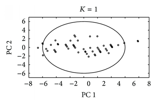
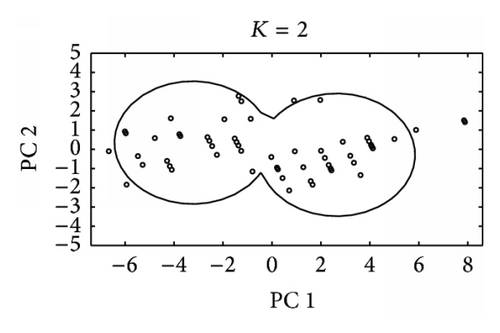
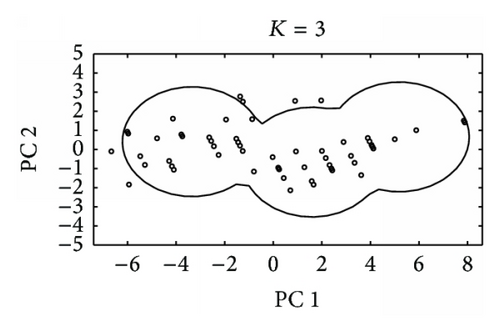
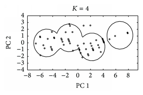
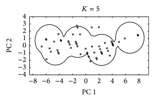
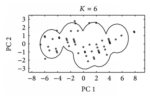
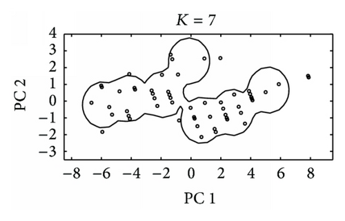
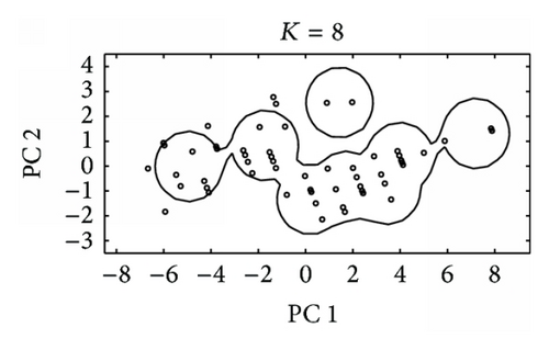
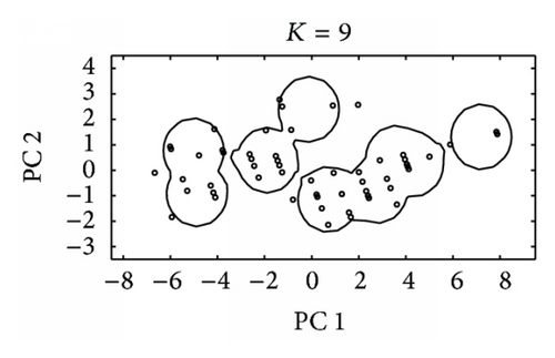
The detection of an abnormal observation in the target class depends on the shape of the established one-class. The KMDD provided a spherical one-class, while SVDD gave a flexible nonspherical one-class due to the use of SVs. It is worth noticing that the shape of SVDD-based one-class depends on the width of the radial basis function while the shape of KNNDD-based one-class is function of the size of the nearest neighbor, denoted by k. Details about the characteristics of SVDD and KNNDD-based one-classes can be found in Gani and Limam [25].

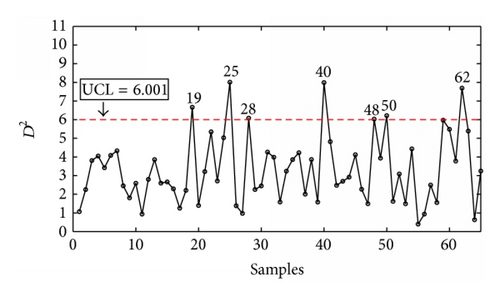
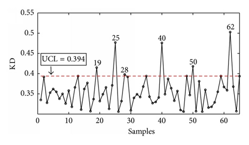
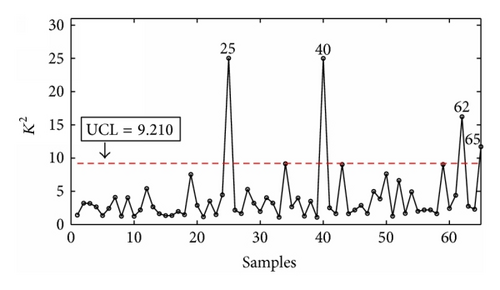
The KM-chart exceeded its control limit of 6.001 at around the 19th, 25th, 28th, 40th, 48th, and 50th cigarettes, as shown in Figure 2. On the other hand, these out-of-control cigarettes have a distance greater than the radius of the established KMDD-based sphere with K = 1. For these six abnormal cigarettes, at least one of their five quality characteristics did not respect its tolerance interval, as discussed above. In comparison with the two other control charts, the proposed KM-chart succeeded to detect a new out-of-control observation which is cigarette number 48. Both K-chart and KNN-chart failed to detect this abnormal cigarette. Once these out-of-control observations are removed, no additional outliers were detected, and the in-control process was established.

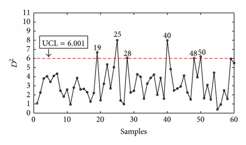
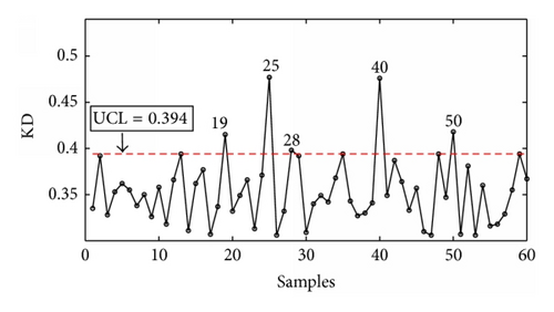
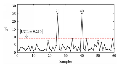
In phase II, five “Cristal Light” cigarettes were used to detect out-of-control states. The KM-chart triggered an alarm at around the 62nd cigarette and remained below its control limit for the last three cigarettes. Cigarette number 62 was also declared by K-chart as an out-of-control observation, while cigarettes number 62 and 65 were declared by KNN-chart as out-of-control observations. Figure 3 shows the discussed OC-charts for phase II.

5. Performance Comparison

In this section, we study the performance of KM-chart and we compare it with K-chart and KNN-chart. The performance study is based on ARL criterion which is defined as the expected number of samples taken before the shift is detected. It is given by

()

where p is the probability of one point plots out-of-control.

A simulation study was conducted to estimate the ARL of OC-charts. In order to be consistent with Gani and Limam [25], we follow their simulation procedure given by the following.

Step 1. Five multivariate normal variables were generated with a mean vector μ = (0.986; 7.650; 0.121; 107.183; 451.527) and a covariance matrix

()

similar to the mean vector and the covariance matrix of the “Cristal Light” data set used in Section 4. The K-chart, KNN-chart, and KM-chart were designed to achieve an overall in-control ARL of 200. The ARL value was estimated by averaging the run lengths obtained by running 1000 simulated charts.

Step 2. Multivariable shifts, denoted by δ, were introduced in the mean vector according to Table 1. Basically, large values of δ correspond to bigger shifts in the mean. The value δ = 0 is the in-control state.

Table 1. ARL comparison for three OC-charts.

δ	K-chart	KNN-chart	KM-chart
0.00	200.000	200.000	200.000
0.25	100.000	200.000	192.308
0.50	66.667	200.000	185.185
0.75	66.667	100.000	166.667
1.00	50.000	40.000	147.059
1.25	50.000	14.285	117.647
1.50	40.000	9.091	86.956
1.75	28.571	3.703	60.976
2.00	22.222	1.695	39.370
2.25	13.333	1.020	25.707
2.50	6.896	1.000	16.340
2.75	4.167	1.000	9.597
3.00	2.439	1.000	5.540
3.25	1.709	1.000	3.250
3.50	1.197	1.000	1.997
3.75	1.036	1.000	1.390
4.00	1.000	1.000	1.116
5.00	1.000	1.000	1.000

For detecting small shifts (δ = 0.25), KM-chart performed better than KNN-chart since it gave an ARL = 192.308, while KNN-chart gave an ARL = 200. For the same shift level, K-chart yielded an ARL = 100, which was better than that of KM-chart.

For detecting moderate shifts (δ = 1), KNN-chart behaved better than the other two control charts since it gave an ARL = 40 against an ARL of 50 and 147.059 of K-chart and KM-chart, respectively.

The difference in sensitivity to shifts in the mean vector between the three OC-charts is due to the difference in the nature of distance used by each control chart. The K-chart uses KD, whereas KM-chart and KNN-chart are based on the Euclidean distance. The advantage of KD in comparison with Euclidean distance lies essentially in the use of the kernel function. The latter is equivalent to the distance between two samples measured in a higher dimensional space. This allows K-chart to easily detect any small shift in the process. In terms of ARL and for small shifts in the mean vector, one can draw the conclusion that our proposed KM-chart is situated between KNN-chart and K-chart (KNN-chart < KM-chart < K-chart). Broadly speaking, each OC-chart has its advantages and disadvantages. For example, K-chart performs better than KM-chart and KNN-chart in quickly detecting changes in the process, while the computational cost of KM-chart and KNN-chart is lower than that of K-chart. Table 2 summarizes the characteristics of each OC-chart.

Table 2. Characteristics of three OC-charts.

	K-chart	KNN-chart	KM-chart
Charting statistic	KD	K²	D²
One-class classifier	SVDD	KNNDD	KMDD
Parameters	RBF’s width σ	The size of nearest neighbor k	The number of clusters K
Distance type	Kernel distance	Euclidean distance	Euclidean distance
Center	Kernel center	KNN center	Cluster center
Suitable cases	Known and unknown distribution	Known and unknown distribution	Known and unknown distribution

6. Conclusion

In this paper, we have developed a new OC-chart using KMDD algorithm, called KM-chart. Construction methodology of KM-chart is demonstrated through a real industrial application. Performance analysis of KM-chart in phase I and II showed that our proposed control chart is a competitive SPC tool. In phase I, the proposed KM-chart detected a new abnormal observation which is cigarette number 48. Both K-chart and KNN-chart failed to detect this abnormal cigarette. Based on the ARL criterion, our proposed control chart outperformed KNN-chart in detecting small shifts in the mean vector.

The proposed KM-chart can be extended to monitor nonlinear processes by using the global kernel K-means algorithm instead of using the standard K-means algorithm. The global kernel K-means has the advantage to identify nonlinearly separable clusters and therefore allows KM-chart to monitor sophisticated manufacturing processes.

Conflict of Interests

The authors declare that they do not have a direct financial relation with the software mentioned in this paper and no competing interests.

Acknowledgment

The authors express their appreciation to LARODEC of ISG, University of Tunis, for supporting this paper.

Appendix

The MATLAB Code for KM-Chart

The MATLAB code for the KM-chart requires the PRtools toolbox available at http://www.prtools.org and the dd_tools toolbox available at http://prlab.tudelft.nl/david-tax/dd_tools.html.

For more details see Algorithm 1.

References

1 Cook D. F., Using basis function networks to recognize shifts in correlated process parameters, IIE Transactions. (1998) 30, no. 3, 227–234, 2-s2.0-0032022864.
10.1080/07408179808966453
Web of Science® Google Scholar
2 Chinnam R. B., Support vector machines for recognizing shifts in correlated and other manufacturing processes, International Journal of Production Research. (2002) 40, no. 17, 4449–4466, 2-s2.0-0037146388, https://doi.org/10.1080/00207540210152920.
10.1080/00207540210152920
Web of Science® Google Scholar
3 Hwang W., Runger G., and Tuv E., Multivariate statistical process control with artificial contrasts, IIE Transactions. (2007) 39, no. 6, 659–669, 2-s2.0-33947689147, https://doi.org/10.1080/07408170600899615.
10.1080/07408170600899615
Web of Science® Google Scholar
4 Hu J., Runger G., and Tuv E., Tuned artificial contrasts to detect signals, International Journal of Production Research. (2007) 45, no. 23, 5527–5534, 2-s2.0-35348913277, https://doi.org/10.1080/00207540701325330.
10.1080/00207540701325330
Web of Science® Google Scholar
5 Gani W., Taleb H., and Limam M., Support vector regression based residual control charts, Journal of Applied Statistics. (2010) 37, no. 2, 309–324, 2-s2.0-75649089278, https://doi.org/10.1080/02664760903002667.
10.1080/02664760903002667
Web of Science® Google Scholar
6 Kim S. B., Jitpitaklert W., Park S.-K., and Hwang S.-J., Data mining model-based control charts for multivariate and autocorrelated processes, Expert Systems with Applications. (2012) 39, no. 2, 2073–2081, 2-s2.0-80054957007, https://doi.org/10.1016/j.eswa.2011.08.010.
10.1016/j.eswa.2011.08.010
Web of Science® Google Scholar
7 Mahadevan S. and Shah S. L., Fault detection and diagnosis in process data using one-class support vector machines, Journal of Process Control. (2009) 19, no. 10, 1627–1639, 2-s2.0-72149111135, https://doi.org/10.1016/j.jprocont.2009.07.011.
10.1016/j.jprocont.2009.07.011
CAS Web of Science® Google Scholar
8 Kim S. B., Jitpitaklert W., and Sukchotrat T., One-class classification-based control charts for monitoring autocorrelated multivariate processes, Communications in Statistics: Simulation and Computation. (2010) 39, no. 3, 461–474, 2-s2.0-77349113379, https://doi.org/10.1080/03610910903480826.
10.1080/03610910903480826
Web of Science® Google Scholar
9 Kittiwachana S., Ferreira D. L. S., Lloyd G. R., Fido L. A., Thompson D. R., Escott R. E. A., and Brereton R. G., One class classifiers for process monitoring illustrated by the application to online HPLC of a continuous process, Journal of Chemometrics. (2010) 24, no. 3-4, 96–110, 2-s2.0-77951066031, https://doi.org/10.1002/cem.1281.
10.1002/cem.1281
CAS Web of Science® Google Scholar
10 Kim S. B., Sukchotrat T., and Park S.-K., A nonparametric fault isolation approach through one-class classification algorithms, IIE Transactions. (2011) 43, no. 7, 505–517, 2-s2.0-79953687096, https://doi.org/10.1080/0740817X.2010.523769.
10.1080/0740817X.2010.523769
Web of Science® Google Scholar
11 Brereton R. G., One-class classifiers, Journal of Chemometrics. (2011) 25, no. 5, 225–246, 2-s2.0-79956325552, https://doi.org/10.1002/cem.1397.
10.1002/cem.1397
CAS Web of Science® Google Scholar
12 Sukchotrat T., Kim S. B., Tsui K.-L., and Chen V. C. P., Integration of classification algorithms and control chart techniques for monitoring multivariate processes, Journal of Statistical Computation and Simulation. (2011) 81, no. 12, 1897–1911.
10.1080/00949655.2010.507765
Web of Science® Google Scholar
13 Tax D. M. J. and Duin R. P. W., Support vector data description, Machine Learning. (2004) 54, no. 1, 45–66, 2-s2.0-0942266514, https://doi.org/10.1023/B:MACH.0000008084.60811.49.
10.1023/B:MACH.0000008084.60811.49
Web of Science® Google Scholar
14 Tax D. M. J., One-class classification: concept-learning in the absence of counter-examples [Ph.D. thesis], 2001, Delft University of Technology, Stevinweg, The Netherlands.
Google Scholar
15 Sun R. and Tsung F., A kernel-distance-based multivariate control chart using support vector methods, International Journal of Production Research. (2003) 41, no. 13, 2975–2989, 2-s2.0-0242333191, https://doi.org/10.1080/1352816031000075224.
10.1080/1352816031000075224
Web of Science® Google Scholar
16 Kumar S., Choudhary A. K., Kumar M., Shankar R., and Tiwari M. K., Kernel distance-based robust support vector methods and its application in developing a robust K-chart, International Journal of Production Research. (2006) 44, no. 1, 77–96, 2-s2.0-29344469347, https://doi.org/10.1080/00207540500216037.
10.1080/00207540500216037
Web of Science® Google Scholar
17 Camci F., Chinnam R. B., and Ellis R. D., Robust kernel distance multivariate control chart using support vector principles, International Journal of Production Research. (2008) 46, no. 18, 5075–5095, 2-s2.0-51749106759, https://doi.org/10.1080/00207540500543265.
10.1080/00207540500543265
Web of Science® Google Scholar
18 Gani W., Taleb H., and Limam M., An assessment of the kernel-distance-based multivariate control chart through an industrial application, Quality and Reliability Engineering International. (2011) 27, no. 4, 391–401, 2-s2.0-79957483540, https://doi.org/10.1002/qre.1117.
10.1002/qre.1117
Web of Science® Google Scholar
19 Gani W. and Limam M., On the use of the K-chart for phase II monitoring of simple linear profiles, Journal of Quality and Reliability Engineering. (2013) 2013, 8, 705450, https://doi.org/10.1155/2013/705450.
10.1155/2013/705450
Google Scholar
20 He S. and Zhang C., Support vector data description based multivariate cumulative sum control chart, Advanced Materials Research. (2011) 314–316, 2482–2485, 2-s2.0-80052977079, https://doi.org/10.4028/www.scientific.net/AMR.314-316.2482.
10.4028/www.scientific.net/AMR.314-316.2482
Web of Science® Google Scholar
21 Ge Z., Gao F., and Song Z., Batch process monitoring based on support vector data description method, Journal of Process Control. (2011) 21, no. 6, 949–959, 2-s2.0-79958136331, https://doi.org/10.1016/j.jprocont.2011.02.004.
10.1016/j.jprocont.2011.02.004
CAS Web of Science® Google Scholar
22 Liu X., Li K., McAfee M., and Irwin G. W., Improved nonlinear PCA for process monitoring using support vector data description, Journal of Process Control. (2011) 21, no. 9, 1306–1317, 2-s2.0-80052565753, https://doi.org/10.1016/j.jprocont.2011.07.003.
10.1016/j.jprocont.2011.07.003
CAS Web of Science® Google Scholar
23 Cho H.-W., Jeong M. K., and Kwon Y., Support vector data description for calibration monitoring of remotely located microrobotic system, Journal of Manufacturing Systems. (2006) 25, no. 3, 196–208, 2-s2.0-59849124858, https://doi.org/10.1016/S0278-6125(07)80009-4.
10.1016/S0278-6125(07)80009-4
Web of Science® Google Scholar
24 Sukchotrat T., Kim S. B., and Tsung F., One-class classification-based control charts for multivariate process monitoring, IIE Transactions. (2010) 42, no. 2, 107–120, 2-s2.0-77649328220, https://doi.org/10.1080/07408170903019150.
10.1080/07408170903019150
Web of Science® Google Scholar
25 Gani W. and Limam M., Performance evaluation of one-class classification-based control charts through an industrial application, Quality and Reliability Engineering International. (2013) 29, no. 6, 841–854.
10.1002/qre.1440
Web of Science® Google Scholar
26 Hajlaoui M., On the charting procedures: T² chart and DD-diagram, International Journal of Quality, Statistics, and Reliability. (2011) 2011, 8, 2-s2.0-84856427287, https://doi.org/10.1155/2011/830764, 830764.
10.1155/2011/830764
Google Scholar

Citing Literature

All articles

A One-Class Classification-Based Control Chart Using the K-Means Data Description Algorithm

Abstract

1. Introduction

2. Background on OC-Charts

2.1. The K-Chart

2.2. The KNN-Chart

3. The Proposed KM-Chart

4. A Real Industrial Application

5. Performance Comparison

6. Conclusion

Conflict of Interests

Acknowledgment

Appendix

The MATLAB Code for KM-Chart

References

Citing Literature

Figures

References

Information

About Wiley Online Library

Help & Support

Opportunities

Connect with Wiley

A One-Class Classification-Based Control Chart Using the K-Means Data Description Algorithm

Abstract

1. Introduction

2. Background on OC-Charts

2.1. The K-Chart

2.2. The KNN-Chart

3. The Proposed KM-Chart

4. A Real Industrial Application

5. Performance Comparison

6. Conclusion

Conflict of Interests

Acknowledgment

Appendix

The MATLAB Code for KM-Chart

References

Citing Literature

Figures

References

Related

Information