For decades, Mackey-Glass chaotic time series prediction has attracted more and more attention. When the multilayer perceptron is used to predict the Mackey-Glass chaotic time series, what we should do is to minimize the loss function. As is well known, the convergence speed of the loss function is rapid in the beginning of the learning process, while the convergence speed is very slow when the parameter is near to the minimum point. In order to overcome these problems, we introduce the Levenberg-Marquardt algorithm (LMA). Firstly, a rough introduction is given to the multilayer perceptron, including the structure and the model approximation method. Secondly, we introduce the LMA and discuss how to implement the LMA. Lastly, an illustrative example is carried out to show the prediction efficiency of the LMA. Simulations show that the LMA can give more accurate prediction than the gradient descent method.

1. Introduction

The Mackey-Glass chaotic time series is generated by the following nonlinear time delay differential equation:

()

where β, γ, τ, and n are real numbers. Depending on the values of the parameters, this equation displays a range of periodic and chaotic dynamics. Such a series has some short-range time coherence, but long-term prediction is very difficult.

Originally, Mackey and Glass proposed the following equation to illustrate the appearance of complex dynamics in physiological control systems by way of bifurcations in the dynamics:

()

They suggested that many physiological disorders, called dynamical diseases, were characterized by changes in qualitative features of dynamics. The qualitative changes of physiological dynamics corresponded mathematically to bifurcations in the dynamics of the system. The bifurcations in the equation dynamics could be induced by changes in the parameters of the system, as might arise from disease or environmental factors, such as drugs or changes in the structure of the system [1, 2].

The Mackey-Glass equation has also had an impact on more rigorous mathematical studies of delay-differential equations. Methods for analysis of some of the properties of delay differential equations, such as the existence of solutions and stability of equilibria and periodic solutions, had already been developed [3]. However, the existence of chaotic dynamics in delay-differential equations was unknown. Subsequent studies of delay differential equations with monotonic feedback have provided significant insight into the conditions needed for oscillation and properties of oscillations [4–6]. For delay differential equations with nonmonotonic feedback, mathematical analysis has proven much more difficult. However, rigorous proofs for chaotic dynamics have been obtained for the differential delay equation dx/dt = g(x(t − 1)) for special classes of the feedback function g [7]. Further, although a proof of chaotic dynamics in the Mackey-Glass equation has still not been found, advances in understanding the properties of delay differential equations is going on, such as (2), that contain both exponential decay and nonmonotonic delayed feedback [8]. The study of this equation remains a topic of vigorous research.

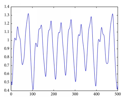
The Mackey-Glass chaotic time series prediction is a very difficult task. The aim is to predict the future state x(t + ΔT) using the current and the past time series x(t), x(t − 1), …, x(t − n) (Figure 2). Until now, there are many literatures about the Mackey-Glass chaotic time series prediction [9–14]. However, as far as the prediction accuracy is concerned, most of the results in the literature are not ideal.

In this paper, we will predict the Mackey-Glass chaotic time series by the MLP. While minimizing the loss function, we introduce the LMA, which can adjust the convergence speed and obtain good convergence efficiency.

The rest of the paper is organized as follows. In Section 2, we describe the multilayer perceptron. Section 3 introduces the LMA and discusses how to implement the LMA. In Section 4, we give a numerical example to demonstrate the prediction efficiency. Section 5 is the conclusions and discussions of the paper.

2. Preliminaries

2.1. Multilayer Perceptrons

A multilayer perceptron (MLP) is a feedforward artificial neural network model that maps sets of input data onto a set of appropriate outputs. A MLP consists of multiple layers of nodes in a directed graph, with each layer fully connected to the next one. Except for the input nodes, each node is a neuron (or processing element) with a nonlinear activation function. The multilayer perceptron with only one hidden layer is depicted as in Figure 1 [15].

Details are in the caption following the image — **Figure 1**
Open in figure viewer PowerPoint

Multilayer Perceptrons.

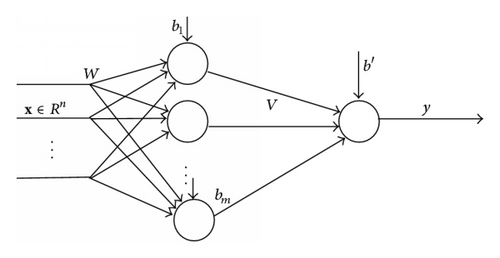
In Figure 1, x = [x₁, x₂, …, x_n] ^T ∈ Rⁿ is the model input, y is the model output, W = {w_ij}, i = 1,2, … , n, j = 1,2, …, m, is the connection weight from the x_i to the jth hidden unit, V = {v_j} is the connection weight from the jth hidden unit to the output unit, b_j, j = 1,2, …, m, and b^′ are the bias.

The output of the multilayer perceptron described in Figure 1 is

()

and the outputs of the hidden units are

()

respectively, where φ(·) is the activation function. We will adopt the sigmoid function φ(x) as the activation function; for example,

()

and the derivative of the activation function with respect to x is

()

MLP provides a universal method for function approximation and classification [16, 17]. In the case of the function approximation, we have a number of observed data (x₁, y₁), (x₂, y₂), …,(x_L, y_L), which are supposed to be generated by

()

where ξ is noise, usually subject to Gaussian distribution with zero mean, and f₀(x) is the unknown true generating function.

Given a set of observed data, sometimes called training examples, we search for the parameters

()

to approximate the teacher function f₀(x) best, where T denotes the matrix transposition. A satisfactory model is often obtained by minimizing the mean square error.

One of the serious problems in minimizing the mean square error is that the convergence speed of the loss function is rapid in the beginning of the learning process, while the convergence speed is very slow in the region of the minimum [18]. In order to overcome these problems, we will introduce the Levenberg-Marquardt algorithm (LMA) in the next section.

2.2. The Levenberg-Marquardt Algorithm

In mathematics and computing, the Levenberg-Marquardt algorithm (LMA) [18–20], also known as the damped least-squares (DLS) method, is used to solve nonlinear least squares problems. These minimization problems arise especially in least squares curve fitting.

The LMA is interpolates between the Gauss-Newton algorithm (GNA) and the gradient descent algorithm (GDA). As far as the robustness is concerned, the LMA performs better than the GNA, which means that in many cases it finds a solution even if it starts very far away from the minimum. However, for well-behaved functions and reasonable starting parameters, the LMA tends to be a bit slower than the GNA.

In many real applications for solving model fitting problems, we often adopt the LMA. However, like many other fitting algorithms, the LMA finds only a local minimum, which is always not the global minimum.

The least squares curve fitting problem is described as follows. Instead of the unknown true model, a set of N pairs of independent variables (x₁, y₁), (x₂, y₂), … , (x_N, y_N) are given. Suppose that f(x, θ) is the approximation model and L(θ) is a loss function, which is the sum of the squares of the deviations:

()

The task of curve fitting problem is minimizing the above loss function L(θ) [21].

The LMA is an iterative algorithm and the parameter θ is adjusted in each iteration step. Generally speaking, we choose an initial parameter randomly, for example, θ_i ~ U(−1,1), i = 1,2, …, n, where n is the dimension of parameter θ.

The Taylor expansion of the function f(x_i, θ + Δθ) is

()

As we know, at the minimum θ^* of loss function L(θ), the gradient of L(θ) with respect to θ will be zero. Substituting (11) into (10), we can obtain

()

where J_i = ∂f(x_i, θ)/∂θ, or

()

Taking the derivative with respect to Δθ and setting the result to zero give

()

where J is the Jacobian matrix whose ith row equals J_i and also y and f are vectors with ith component f(x_i, θ) and y_i, respectively. This is a set of linear equations which can be solved for Δθ.

Levenberg’s contribution is to replace this equation by a “damped version,”

()

where I is the identity matrix, giving the increment Δθ to the estimated parameter vector θ.

The damping factor λ is adjusted at each iteration step. If the loss function L(θ) reduces rapidly, λ will adopt a small value, and then the LMA is similar to the Gauss-Newton algorithm. While the loss function L(θ) reduces very slowly, λ can be increased, giving a step closer to the gradient descent direction, and

()

Therefore, for large values of λ, the step will be taken approximately in the direction of the gradient.

In the process of iteration, if either the length of the calculated step Δθ or the reduction of L(θ) from the latest parameter vector θ + Δθ falls below the predefined limits, iteration process stops and then we take the last parameter vector θ as the final solution.

Levenberg’s algorithm has the disadvantage that if the value of damping factor λ is large, the inverse of J^TJ + λI does not work at all. Marquardt provided the insight that we can scale each component of the gradient according to the curvature so that there is larger movement along the directions where the gradient is smaller. This avoids slow convergence in the direction of small gradient. Therefore, Marquardt replaced the identity matrix I with the diagonal matrix consisting of the diagonal elements of J^TJ, resulting in the Levenberg-Marquardt algorithm [22]:

()

and the LMA is as follows:

()

where

()

3. Application of LMA for Mackey-Glass Chaotic Time Series

In this section, we will derive the LMA when the MLP is used for the Mackey-Glass chaotic time series prediction. Suppose that we use the x(t) − ΔT₀, x(t − ΔT₁), … , x(t − ΔT_n−1) to predict the future variable x(t + ΔT), where ΔT₀ = 0.

To implement the LMA, what we should do is calculate the Jacobian matrix J, whose ith row equals J_i. According to (3) and (4), function f(x, θ) can be expressed as

()

What we should do is calculate the J_i = ∂f(x_i, θ)/∂θ.

The derivatives of f(x, θ) with respect to θ are

()

As we know, θ = (b₁, …, b_m, w₁₁, …, w_n1, w₁₂, …, w_n2, … , w_1m, …, w_nm, b^′, v₁, …, v_m) ∈ R^(n+1)m+m+1, so J_i, the ith row of J, can be easily obtained according to (21). J is calculated and when MLP is used for Mackey-Glass chaotic time series prediction, the LMA can also be obtained.

4. Numerical Simulations

Example 1. We will conduct an experiment to show the efficiency of the Levenberg-Marquardt algorithm. We choose a chaotic time series created by the Mackey-Glass delay-difference equation:

()

for τ = 17.

Such a series has some short-range time coherence, but long-term prediction is very difficult. The need to predict such a time series arises in detecting arrhythmias in heartbeats.

The network is given no information about the generator of the time series and is asked to predict the future of the time series from a few samples of the history of the time series. In our example, we trained the network to predict the value at time T + ΔT, from inputs at time T, T − 6, T − 12, and T − 18, and we will adopt ΔT = 50 here.

In the simulation, 3000 training examples and 500 test examples are generated by (22). We use the following multilayer perceptron for fitting the generated training examples:

()

for example, the number of the hidden units is n = 20 and the dimension of the input is m = 4.

Let ; then, we can obtain the following equation according to (21):

()

The initial values of the parameters are selected randomly:

()

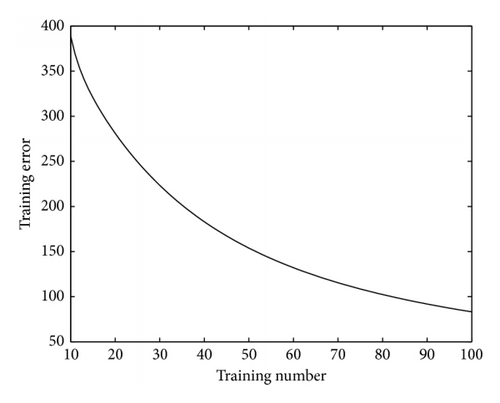
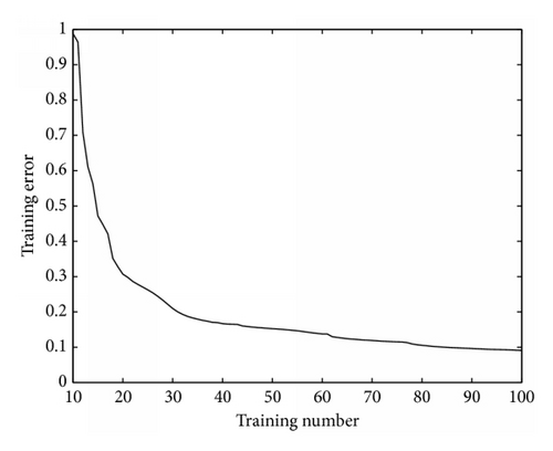
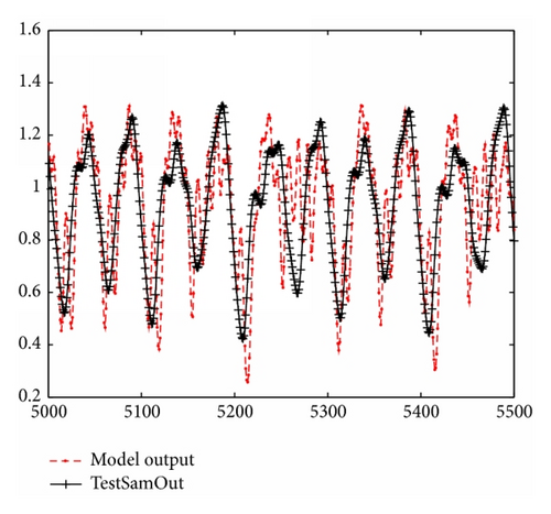
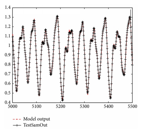
The learning curves of the error function and the fitting result of LMA and GDA are shown in Figures 3, 4, 5, and 6, respectively.

The learning curves of LMA and GNA are shown in Figures 3 and 4, respectively. The training error of LMA can reach 0.1, while the final training error of GDA is more than 90. Furthermore, the final mean test error of LMA is much smaller than 0.2296, which is the final test error of GDA.

As far as the fitting effect is concerned, the performance of LMA is much better than that of the GDA. This is very obvious from Figures 5 and 6.

All of these suggest that when we predict the Mackey-Glass chaotic time series, the performance of LMA is very good. It can effectively overcome the difficulties which may arise in the GDA.

5. Conclusions and Discussions

In this paper, we discussed the application of the Levenberg-Marquardt algorithm for the Mackey-Glass chaotic time series prediction. We used the multilayer perceptron with 20 hidden units to approximate and predict the Mackey-Glass chaotic time series. In the process of minimizing the error function, we adopted the Levenberg-Marquardt algorithm. If reduction of L(θ) is rapid, a smaller value damping factor λ can be used, bringing the algorithm closer to the Gauss-Newton algorithm, whereas if an iteration gives insufficient reduction in the residual, λ can be increased, giving a step closer to the gradient descent direction. In this paper, the learning mode is batch. At last, we demonstrate the performance of the LMA. Simulations show that the LMA can achieve much better prediction efficiency than the gradient descent method.

Conflict of Interests

The authors declare that there is no conflict of interests regarding the publication of this paper.

Acknowledgment

This project is supported by the National Natural Science Foundation of China under Grants 61174076, 11471152, and 61403178.

References

1 Mackey M. C. and Glass L., Oscillation and chaos in physiological control systems, Science. (1977) 197, no. 4300, 287–289, https://doi.org/10.1126/science.267326, 2-s2.0-0017714604.
10.1126/science.267326
CAS PubMed Web of Science® Google Scholar
2 Glass L. and Mackey M. C., Mackey-Glass equation, Scholarpedia. (2010) 5, no. 3.
10.4249/scholarpedia.6908
PubMed Google Scholar
3 Hale J., Theory of Functional Differential Equations, 1977, Springer, New York, NY, USA, MR0508721.
10.1007/978-1-4612-9892-2
Web of Science® Google Scholar
4 Mallet-Paret J. and Nussbaum R. D., A differential-delay equation arising in optics and physiology, SIAM Journal on Mathematical Analysis. (1989) 20, no. 2, 249–292, https://doi.org/10.1137/0520019, MR982660, ZBL0676.34043.
10.1137/0520019
Web of Science® Google Scholar
5 Walther H. O., The 2-dimensional attractor of dx/dt = μx(t) + f(x(t − 1)), Memoirs of the American Mathematical Society. (1995) 113, no. 544.
Web of Science® Google Scholar
6 Mallet-Paret J. and Sell G. R., The Poincaré-Bendixson theorem for monotone cyclic feedback systems with delay, Journal of Differential Equations. (1996) 125, no. 2, 441–489, https://doi.org/10.1006/jdeq.1996.0037, MR1378763, 2-s2.0-0030102885.
10.1006/jdeq.1996.0037
Web of Science® Google Scholar
7 Lani-Wayda B. and Walther H.-O., Chaotic motion generated by delayed negative feedback, part II: construction of nonlinearities, Mathematische Nachrichten. (2000) 180, 181–211.
Google Scholar
8 Röst G. and Wu J. H., Domain-decomposition method for the global dynamics of delay differential equations with unimodal feedback, Proceedings of The Royal Society of London. Series A. Mathematical, Physical and Engineering Sciences. (2007) 463, no. 2086, 2655–2669, https://doi.org/10.1098/rspa.2007.1890, MR2352875, 2-s2.0-36348976487.
10.1098/rspa.2007.1890
Web of Science® Google Scholar
9 Awad M., Pomares H., Rojas I., Salameh O., and Hamdon M., Prediction of time series using RBF neural networks: a new approach of clustering, International Arab Journal of Information Technology. (2009) 6, no. 2, 138–143, 2-s2.0-79958122412.
Web of Science® Google Scholar
10 Awad M., Chaotic time series prediction using wavelet neural network, Journal of Artificial Intelligence: Theory and Application. (2010) 1, no. 3, 73–80.
Google Scholar
11 López-Yáñez I., Sheremetov L., and Yáñez-Márquez C., A novel associative model for time series data mining, Pattern Recognition Letters. (2014) 41, 23–33, https://doi.org/10.1016/j.patrec.2013.11.008.
10.1016/j.patrec.2013.11.008
Web of Science® Google Scholar
12 Fowler A. C., Respiratory control and the onset of periodic breathing, Mathematical Modelling of Natural Phenomena. (2014) 9, no. 1, 39–57, https://doi.org/10.1051/mmnp/20149104, MR3177828, 2-s2.0-84893912572.
10.1051/mmnp/20149104
Web of Science® Google Scholar
13 Wang N., Er M. J., and Han M., Generalized single-hidden layer feedforward networks for regression problems, IEEE Transactions on Neural Networks and Learning Systems. (2014) https://doi.org/10.1109/TNNLS.2014.2334366.
10.1109/TNNLS.2014.2334366
Web of Science® Google Scholar
14 Wang N., A generalized ellipsoidal basis function based online self-constructing fuzzy neural network, Neural Processing Letters. (2011) 34, no. 1, 13–37, https://doi.org/10.1007/s11063-011-9181-1, 2-s2.0-80052654802.
10.1007/s11063-011-9181-1
Web of Science® Google Scholar
15 Wei H. K., Theory and Method of the Neural Networks Architecture Design, 2005, National Defence Industry Press, Beijing, China.
Google Scholar
16 Wei H. and Amari S.-I., Dynamics of learning near singularities in radial basis function networks, Neural Networks. (2008) 21, no. 7, 989–1005, https://doi.org/10.1016/j.neunet.2008.06.017, 2-s2.0-51049114453.
10.1016/j.neunet.2008.06.017
PubMed Web of Science® Google Scholar
17 Wei H., Zhang J., Cousseau F., Ozeki T., and Amari S.-I., Dynamics of learning near singularities in layered networks, Neural Computation. (2008) 20, no. 3, 813–843, https://doi.org/10.1162/neco.2007.12-06-414, MR2382962, 2-s2.0-41549141920.
10.1162/neco.2007.12-06-414
PubMed Web of Science® Google Scholar
18 Levenberg K., A method for the solution of certain non-linear problems in least squares, Quarterly of Applied Mathematics. (1944) 2, 164–168, MR0010666, ZBL0063.03501.
10.1090/qam/10666
Google Scholar
19 Hagan M. T. and Menhaj M. B., Training feedforward networks with the Marquardt algorithm, IEEE Transactions on Neural Networks. (1994) 5, no. 6, 989–993, https://doi.org/10.1109/72.329697, 2-s2.0-0028543366.
10.1109/72.329697
CAS PubMed Web of Science® Google Scholar
20 Guo W., Wei H., Zhao J., and Zhang K., Averaged learning equations of error-function-based multilayer perceptrons, Neural Computing and Applications. (2014) 25, no. 3-4, 825–832, https://doi.org/10.1007/s00521-014-1557-5, 2-s2.0-84893930950.
10.1007/s00521-014-1557-5
Web of Science® Google Scholar
21 Gill P. E. and Murray W., Algorithms for the solution of the nonlinear least-squares problem, SIAM Journal on Numerical Analysis. (1978) 15, no. 5, 977–992, https://doi.org/10.1137/0715063, MR507558, ZBL0401.65042.
10.1137/0715063
Web of Science® Google Scholar
22 Marquardt D. W., An algorithm for least-squares estimation of nonlinear parameters, SIAM Journal on Applied Mathematics. (1963) 11, no. 2, 431–441, MR0153071.
10.1137/0111030
CAS Web of Science® Google Scholar

Citing Literature

All articles

Levenberg-Marquardt Algorithm for Mackey-Glass Chaotic Time Series Prediction

Abstract

1. Introduction

2. Preliminaries

2.1. Multilayer Perceptrons

2.2. The Levenberg-Marquardt Algorithm

3. Application of LMA for Mackey-Glass Chaotic Time Series

4. Numerical Simulations

5. Conclusions and Discussions

Conflict of Interests

Acknowledgment

References

Citing Literature

Figures

References

Information

About Wiley Online Library

Help & Support

Opportunities

Connect with Wiley

Levenberg-Marquardt Algorithm for Mackey-Glass Chaotic Time Series Prediction

Abstract

1. Introduction

2. Preliminaries

2.1. Multilayer Perceptrons

2.2. The Levenberg-Marquardt Algorithm

3. Application of LMA for Mackey-Glass Chaotic Time Series

4. Numerical Simulations

5. Conclusions and Discussions

Conflict of Interests

Acknowledgment

References

Citing Literature

Figures

References

Related

Information