Solving Continuous Models with Dependent Uncertainty: A Computational Approach
Abstract
This paper presents a computational study on a quasi-Galerkin projection-based method to deal with a class of systems of random ordinary differential equations (r.o.d.e.’s) which is assumed to depend on a finite number of random variables (r.v.’s). This class of systems of r.o.d.e.’s appears in different areas, particularly in epidemiology modelling. In contrast with the other available Galerkin-based techniques, such as the generalized Polynomial Chaos, the proposed method expands the solution directly in terms of the random inputs rather than auxiliary r.v.’s. Theoretically, Galerkin projection-based methods take advantage of orthogonality with the aim of simplifying the involved computations when solving r.o.d.e.’s, which means to compute both the solution and its main statistical functions such as the expectation and the standard deviation. This approach requires the previous determination of an orthonormal basis which, in practice, could become computationally burden and, as a consequence, could ruin the method. Motivated by this fact, we present a technique to deal with r.o.d.e.’s that avoids constructing an orthogonal basis and keeps computationally competitive even assuming statistical dependence among the random input parameters. Through a wide range of examples, including a classical epidemiologic model, we show the ability of the method to solve r.o.d.e.’s.
1. Introduction and Motivation
The nondeterministic nature of phenomena in areas such as engineering, physics, chemistry, and epidemiology often leads to mathematical continuous models formulated by random ordinary differential equations (r.o.d.e.’s). The uncertainty involving such phenomena appears through the input model parameters (coefficients, source/forcing term, initial/boundary conditions) which then are considered as random variables (r.v.’s) and stochastic processes (s.p.’s) rather than constants and ordinary functions, respectively. The complexity of such stochastic continuous models becomes greater when random inputs are assumed to be statistically dependent, a hypothesis that is met in practice.
Solving a r.o.d.e. consists of not only computing its solution, which is a s.p., but also its main statistical characteristics such as the mean and standard deviation/variance functions. To achieve these objectives, a high number of methods have been proposed, although we underline that most of them rely on the statistical independence of the random input parameters. A good account of such methods can be found in [1].
Now, we remark some aspects related to gPC that will help to highlight better the differences with the method that will be presented in the next section. In dealing with r.o.d.e.’s which depend on a number of random parameters, (ζ1, ζ2, …, ζs), in general, gPC method represents these parameters as well as the solution s.p., y(t), in terms of a family of r.v.’s, ξ = (ξ1, ξ2, …) rather than directly in terms of the random inputs: ζi, 1 ≤ i ≤ s. The selection of r.v.’s ξj as well as the orthogonal basis {Φk(ξ)} must be made according to the probability distributions of the random inputs ζi. In [3], authors provide a comprehensive criterion to set this choice in such a way that an exponential convergence of the error measures for the average and variance of the approximations of the solution holds. In [3], the usefulness of this guideline is shown when there is just one random input parameter, and it also belongs to some of the standard distributions (Poisson, binomial, gaussian, beta, exponential, etc.). In the usual case that two or more r.v.’s appear as input parameters, none of optimal criteria have been established, even assuming that the involved r.v.’s have standard probabilistic distributions.
From a theoretical point of view, the orthogonality of the basic functions used in the previous development permits to cancel some involved computations (inner products) when setting the deterministic system of o.d.e.’s (4), although in practice, the total number of cancelations depends strongly on the specific form of the r.o.d.e. (1). However, this theoretical advantage may not compensate the high computational cost that usually entails the orthogonalization process. Moreover, orthogonalization is a critical part of the process, and the obtained result may return vectors with loss of orthogonality what may ruin the computations of the involved inner products and the building and resolution of system (4), [8, pp.230–232] Golub. This leads us to present a method, based on the Galerkin projection, that overcomes this drawback. The study focuses on computational aspects.
The paper is organized as follows. In Section 2, we present the Galerkin projection-based method that allows us to solve a certain class of systems of r.o.d.e.’s whose uncertainty is considered through a finite number of dependent r.v.’s. Expressions for the expectation and the variance of the solution s.p. are also given. Section 3 is addressed to present the algorithm of the method proposed in Section 2 as well as to discuss its most relevant computational aspects. Section 4 begins with a test example whose exact expressions for the mean and variance are available. Hence, the quality of the approximations provided by the proposed method is better assessed. This comparative study is completed by showing the competitiveness of our approach against the Monte-Carlo simulations. The rest of the section is devoted to show a wide range of examples, for both r.o.d.e.’s and systems of r.o.d.e.’s, where the proposed method is satisfactorily applied. In all these examples, the randomness is also considered through different joint probability distributions to illustrate better the power of the proposed method. Conclusions are drawn in Section 5.
2. Method
As in this paper, we are concerned with constructive computational aspects, and we will assume that conditions for the existence and uniqueness of a solution stochastic process to initial value problem (6) are satisfied. We point out that the available results mainly consist of a natural generalization of the classical Picard theorem based upon convergence in the space L2 of successive approximations [1, page 118].
Remark 1. For the sake of clarity in the presentation, we have used the multi-index notation (i1, …, is) to express the polynomial basis , being as with i1 + ⋯+is = k, 0 ≤ k ≤ m. As a consequence, we have represented the solution s.p. y(t) in the form (8) rather than (1), where , with P = (s + m)!/s! m! − 1, is the elements of the correspondent basis. However, notice that both expressions are equivalent except for orthogonality. In fact, writing ζ instead of ξ (since now we are directly using the vector random models parameters to represent the solution), this identification can be checked considering the following simple tensor product:
3. Algorithm
Based on the method previously developed, in this section, we will give an algorithm to compute the expectation and the standard deviation of the solution s.p. of a random i.v.p. of the form (6) whose analytical expressions are given by (15)-(16), respectively.
- (i)
the r.o.d.e.’s (model): , with random initial condition: y(t0, ζ) = y0;
- (ii)
the random model parameters (this includes both the coefficients/forcing terms of the r.o.d.e. and the initial conditions): ζ = (ζ1, …, ζs);
- (iii)
the joint probability density function (p.d.f.) of ζ: fζ(ζ);
- (iv)
the truncation order m of the polynomial expansion of random model parameters (see expression (7)).
- (i)
Step 1. Define the scalar product 〈 , 〉 given by (11).
- (ii)
Step 2. Build the basis ℬs,m of canonical polynomials of degree ≤m of the s random model parameters, as given in (7).
- (iii)
Step 3. Consider the truncated expansions to the solution s.p., its derivative, and the random initial condition given by (8), (9), and (13), respectively.
- (iv)
Step 4. Substitute the above expansions into the model to obtain the random i.v.p. (10) and (13).
- (v)
Step 5. Obtain the auxiliary system in two phases: first, multiplying each equation of the random i.v.p. (10) and (13) by the polynomials of the basis built in Step 2 and, second, taking the ensemble average inferred by the inner product 〈 , 〉 constructed in Step 1. In this manner, expressions (12) and (14) are obtained, respectively.
- (vi)
Step 6. Solve numerically the auxiliary system set in Step 5.
- (vii)
Step 7. Compute the expectation and the standard deviation (or equivalently, the variance) of the solution s.p. y(t) taking into account expressions in (15) and (16).
3.1. Computational Aspects and Implementation
The algorithm has been implemented using Mathematica [9], and it is available at http://gpcdep.imm.upv.es. We have used symbolic manipulation features of this computational software program to optimise the algorithm performance. Therefore, even though the natural implementation order seems to be the one shown in the presented algorithm, we have decided to implement a symbolic version of Steps 1, 3, 4 and 5 as the first step, where all the inner products have been decomposed into auxiliary inner products as in (19), and these new inner products have not been carried out (they have been manipulated symbolically). Doing this, we have realised that a lot of the inner products are repeated. In fact, regarding Examples 2–8 of Section 4 only around 2%–20% of them are different, what implied an important computational saving in the most critical step. The more independence in the r.v.’s, the more saving, because the inner products corresponding to independent r.v.’s can be computed separately. Table 1 collects the percentages of computational saving related to the involved inner products in the examples shown in Section 4.
| Example | No. theoretical 〈, 〉 | No. computed 〈, 〉 | % of computational saving |
|---|---|---|---|
| 2 | 468 | 62 | 86.75% |
| 3 | 177 | 34 | 80.79% |
| 4 | 2484 | 255 | 89.73% |
| 5 | 9905 | 827 | 91.65% |
| 6 | 1615 | 260 | 83.90% |
| 7 | 249 | 51 | 79.51% |
| 8 | 5745 | 68 | 98.82% |
Once the auxiliary system has been stated symbolically, we define the inner product and try to use the simplification commands provided by Mathematica to obtain the inner product (19) in a form that can be computed faster. It is used to be easy when the inner product is defined in a bounded domain. In unbounded domains, simplification is often no possible, and the computation of the inner products turns difficult to be carried out when the degree of the polynomial increases.
Then, we compute the nonrepeated inner products of the form (19) appearing into the auxiliary system. We must point out that this is the most demanding step.
Next, we substitute the obtained inner products into the auxiliary system, which is then solved numerically using NDSolve command. Finally, the expectation and the standard deviation are computed.
4. Examples
The two first ones are test examples since their exact solutions are available. Then, the quality of the approximations provided by our approach can be better assessed. In the former, we will compare the approximations provided by our approach with the ones corresponding to Monte-Carlo simulations. Monte-Carlo technique can be considered as the most commonly approach used to deal with r.o.d.e.’s. In the second test example, we will detail all the involved computations to clarify the previous notation and methodology.
In Example 7, we illustrate the technique using another r.o.d.e. Finally, we complete the study examples showing the ability of the proposed technique to deal with a classical SIRS-epidemiological model.
The Mathematica source code, its explanation and application to solve Examples 1–7 can be found at http://gpcdep.imm.upv.es.
Example 1. Let us consider the linear r.o.d.e. as follows:
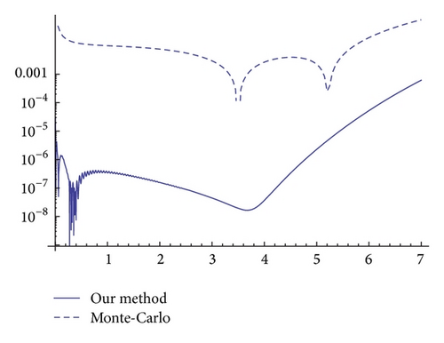
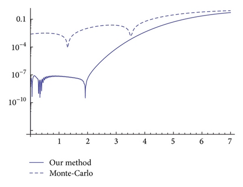
In order to illustrate the competitiveness of the proposed method against Monte-Carlo simulations, in Figures 1 and 2 we show their relative errors with respect to the exact expectation and standard deviation on the interval [0,7], respectively. To highlight better the differences, a logarithmic scale has been used in the vertical axis in both plots. In accordance with the notation introduced in the previous section, the approximations to both statistical moments have been carried out having the following: q = 1, s = 2, and m = 10 (i.e., polynomials of degree equal to or less than 10 have been used), whereas the Monte-Carlo approximations have been performed using 105 simulations. These plots show that the proposed method provides very good approximations which improve the ones generated by Monte-Carlo technique.
Example 2. Let us consider the r.o.d.e. as follows:
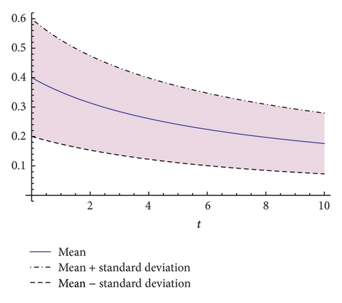
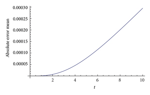
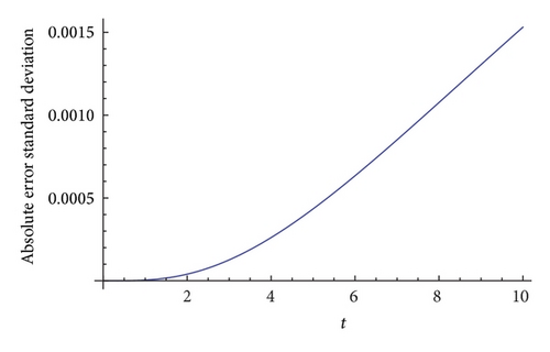
The quality of the approximations to the expectation and the standard deviation can be assessed in this example since the corresponding exact expressions are available. Figures 4(a) and 4(b) show the absolute errors for the approximations to the expectation and the standard deviation of the solution s.p. y(t) on the interval [0,10], respectively. Both plots show that the approximations provided by the method presented in Section 2 are reliable.
Example 3. Let us consider the following r.o.d.e. based on (20) where now uncertainty appears through the two coefficients ζ2 and ζ3:
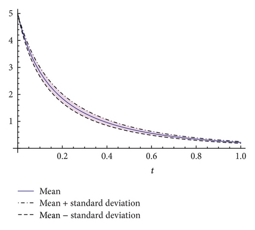
Example 4. Now, we analyse the r.o.d.e. (20) where randomness is considered through three random parameters. Specifically, let the random i.v.p. be as follows:

Example 5. In this example, we deal with r.o.d.e. (20) assuming that uncertainty appears through all the parameters ζi, 1 ≤ i ≤ 4. We will assume that the random vectors ζ1 = (ζ4, ζ1) and ζ2 = (ζ2, ζ3) have multivariate Gaussian distributions; that is, , i = 1,2, where
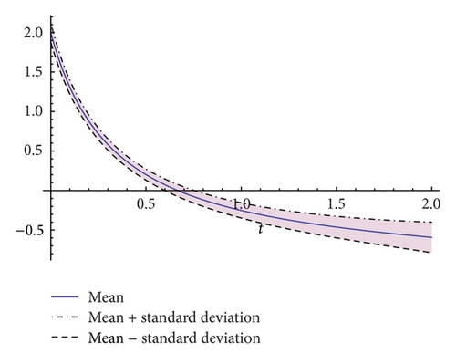
Example 6. In this example, we deal with r.o.d.e. (20) assuming that uncertainty appears through all the parameters ζi, 1 ≤ i ≤ 4. We will assume that the random vector ζ = (ζ1, ζ2, ζ3, ζ4) has a multivariate Gaussian distribution; that is, ζ : N(μζ; Σζ), where
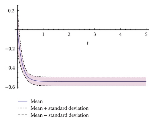
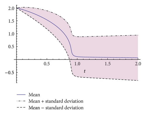
Example 7. In this example we will study the following nonlinear r.o.d.e.:
Example 8. In this example, we consider the SIRS (Susceptible-Infectious-Recovered-Susceptible) model for the transmission of dynamics of the Respiratory Syncitial Virus (RSV) proposed by Weber et al. in [10]. This model is based on the following nonautonomous system of differential equations:
In [10], the authors study the spread of RSV in Finland, obtaining the following parameter values: μ = 0.013; γ = 360/200 = 1.8; ν = 36; b0 = 44; b1 = 0.36; ϕ = 0.6. We will assume that the random vectors ζ1 = (γ, ν) and ζ2 = (b0, b1) have bivariate Gaussian distributions; that is, , i = 1,2, where
Now, we assume that 1% of total population is infectious, so initial conditions are given by S0 = 0.99, I0 = 0.01, and R0 = 0.
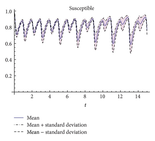
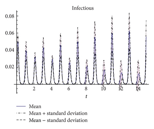
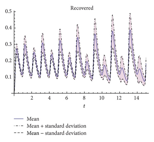
In Figures 10, 11, and 12 we have plotted the approximations of the expectation (solid line) and plus/minus the standard deviation (dashed lines) of the susceptible (S(t)), infected (I(t)), and recovered (R(t)), respectively, on the time-interval [0,15]. These approximations have been computed using (4 + 2)!/(4! 2!) = 15 polynomials of degree equal to or less than 2. Notice that according to the previous notation one has q = 3, s = 4, and m = 2.
5. Conclusions
In this paper, we have presented a method to deal with dependent randomness into a class of continuous models (systems of random ordinary differential equations) focusing on computational aspects and its applicability to a wide range of examples. The method shares similarities with generalized polynomial chaos (gPC) in its basics since it is based on a variation of Galerkin projection techniques. However, the first main difference with respect to gPC approach is that it represents both the random model inputs as well as the solution stochastic process directly in terms of the random model parameters; therefore, accurate approximations of the expectation and standard deviation of the solution are provided. Second, the method avoids constructing an orthogonal basis to set such representations. In this manner, one of the computational bottlenecks to gPC, which is the construction of the so-called auxiliary system (see expressions (12)–(14)) from the orthogonal basis, is avoided. Finally, we have shown through a wide variety of examples the ability of the method to deal successfully with random continuous models whose uncertainty is given by statistical dependent random variables, which is the most complex situation.
Acknowledgments
This work has been partially supported by the Spanish M.C.Y.T. Grants: DPI2010-20891-C02-01 and FIS PI-10/01433; the Universitat Politècnica de València Grant: PAID06-11-2070, and the Universitat de València Grant: UV-INV-PRECOMP12-80708.


