We extend the classical SIRS epidemic model incorporating media coverage from a deterministic framework to a stochastic differential equation (SDE) and focus on how environmental fluctuations of the contact coefficient affect the extinction of the disease. We give the conditions of existence of unique positive solution and the stochastic extinction of the SDE model and discuss the exponential p-stability and global stability of the SDE model. One of the most interesting findings is that if the intensity of noise is large, then the disease is prone to extinction, which can provide us with some useful control strategies to regulate disease dynamics.

1. Introduction

Recent years, a number of mathematical models have been formulated to describe the impact of media coverage on the dynamics of infectious diseases [1–10]. Mass media (television, radio, newspapers, billboards, and booklets) has been used as a way of delivering preventive health messages as it has the potential to influence people’s behavior and deter them from risky behavior or from taking precautionary measures in relation to a disease outbreak [7, 11, 12]. Hence, media coverage has an enormous impact on the spread and control of infectious diseases [2, 3, 9].

On the other hand, for human disease, the nature of epidemic growth and spread is inherently random due to the unpredictability of person-to-person contacts [13], and population is subject to a continuous spectrum of disturbances [14, 15]. In epidemic dynamics, stochastic differential equation (SDE) models could be the more appropriate way of modeling epidemics in many circumstances and many realistic stochastic epidemic models can be derived based on their deterministic formulations [16–28].

In [10], Liu investigated an SIRS epidemic model incorporating media coverage with random perturbation. He assumed that stochastic perturbations were of white noise type, which were directly proportional to distance susceptible S(t), infectious I(t), and recover R(t) from values of endemic equilibrium point (S^*, I^*, R^*), influence on the dS(t)/dt, dI(t)/dt, dR(t)/dt, respectively. In fact, besides the possible equilibrium approach in [10], there are different possible approaches to introduce random effects in the epidemic models affected by environmental white noise from biological significance and mathematical perspective [28–30]. Some scholars [17, 28, 30, 31] demonstrated that one or more system parameter(s) can be perturbed stochastically with white noise term to derive environmentally perturbed system.

In [10], the author proved that the endemic equilibrium of the stochastic model is asymptotically stable in the large. Therefore, it is natural to ask how environmental fluctuations of the contact coefficient affect the extinction of the disease.

In this paper, we will focus on the effects of environmental fluctuations on the disease’s extinction through studying the stochastic dynamics of an SIRS model incorporating media coverage. The rest of this paper is organized as follows. In Section 2, based on the results of Cui et al. [2] and [10], we derive the stochastic differential SIRS model incorporating media coverage. In Section 3, we give the conditions of existence of unique positive solution and the stochastic extinction of the SDE model. In Section 4, we provide some examples to support our research results. In the last section, we provide a brief discussion and the summary of main results.

2. Model Derivation and Related Definitions

2.1. Model Derivation

Let S(t) be the number of susceptible individuals, I(t) the number of infective individuals, and R(t) the number of removed individuals at time t, respectively. Based on the work of Cui et al. [2] and [10], we consider the SIRS epidemic model incorporating media coverage as follows:

(1)

where Λ is the recruitment rate, μ represents the natural death rate, η is the loss of constant immunity rate, α is the diseases induced constant death rate, and λ is constant recovery rate. β₁ is the usual contact rate without considering the infective individuals and β₂ is the maximum reduced contact rate due to the presence of the infected individuals. No one can avoid contacting with others in every case, so it is assumed that β₁ > β₂. The half-saturation constant b > 0 reflects the impact of media coverage on the contact transmission. The function I/(b + I) is a continuous bounded function which takes into account disease saturation or psychological effects.

For model (1), the basic reproduction number

(2)

is the threshold of the system for an epidemic to occur. Model (1) has a disease-free equilibrium E₀ = (Λ/μ, 0,0) and the endemic equilibrium if R₀ > 1. The disease-free equilibrium is globally asymptotically stable if R₀ ≤ 1 and unstable if R₀ > 1. The endemic equilibrium is globally asymptotically stable if R₀ > 1. These results of model (1) were studied in [10].

If we replace the contact rate β₁ in model (1) by β₁ + σ(dB/dt), where dB/dt is a white noise (i.e., B(t) is a Brownian motion), model (1) becomes as follows:

(3)

Obviously, the stochastic model (3) has the same disease-free equilibrium E₀ = (Λ/μ, 0,0) as model (1).

Throughout this paper, let (Ω, ℱ, ℙ) be a complete probability space with a filtration

satisfying the usual conditions (i.e., it is right continuous and increasing while ℱ₀ contains all ℙ-null sets). Define a bounded set Γ as follows:

(4)

2.2. Related Definitions

Consider the general n-dimensional stochastic differential equation

(5)

on t ≥ 0 with initial value x(0) = x₀, the solution is denoted by x(t, x₀). Assume that f(0, t) = 0 and φ(0, t) = 0 for all t ≥ 0, so (5) has the solution x(t) = 0, which is called the trivial solution.

Let us first recall a few definitions.

Definition 1 (see [32].)The trivial solution x(t) = 0 of (5) is said to be

(i)
stable in probability if, for all ɛ > 0,
(6)
(ii)
asymptotically stable if it is stable in probability and moreover if
(7)
(iii)
globally asymptotically stable if it is stable in probability and moreover if, for all x₀ ∈ ℝⁿ
(8)
(iv)
almost surely exponentially stable if for all x₀ ∈ ℝⁿ,
(9)
(v)
exponentially p-stable if there is a pair of positive constants C₁ and C₂ such that for all x₀ ∈ ℝⁿ,
(10)

3. Dynamics of the SDE Model (3)

In what follows, we first use the method of Lyapunov functions to find conditions of existence of unique positive solution of model (3).

3.1. Existence of Unique Positive Solution of Model (3)

In this subsection, we show the existence of the unique positive global solution of SDE model (3).

Theorem 2. Consider model (3), for any given initial value (S(0), I(0), R(0)) ∈ Γ; then there is a unique solution (S(t), I(t), R(t)) on t ≥ 0 and it will remain in with probability one.

Proof. The proof is almost identical to Theorem 2 of [33], but for completeness we repeat it here. Let (S(0), I(0), R(0)) ∈ Γ. Summing up the three equations in (3) and denoting N(t) = S(t) + I(t) + R(t), we have

(11)

Then, if

for all 0 ≤ s ≤ t almost surely (briefly a.s.), we get

(12)

Hence, by integration, we check

(13)

Then, 0 < Λ/(μ + α) < N(s) < Λ/μ a.s., so,

(14)

Since the coefficients of model (3) satisfy the local Lipschitz condition, there is a unique local solution on [0, τ_e), where τ_e is the explosion time. Therefore, the unique local solution to model (3) is positive by the Itô’s formula. Now, let us show that this solution is global; that is, τ_e = ∞ a.s.

Let ϵ₀ > 0 such that S(0), I(0), R(0) > ϵ₀. For ϵ ≤ ϵ₀, define the stop-times

(15)

Then

(16)

Define a C²-function by

(17)

By the Itô’s formula, for all t ≥ 0, s ∈ [0, t∧τ_ϵ], we obtain

(18)

where

(19)

By (14) we assert that (S(s), I(s), R(s))∈(0, Λ/μ) for all s ∈ [0, t∧τ_ϵ] a.s. Hence

(20)

Substituting this inequality into (18), we see that

(21)

which implies that

(22)

Taking the expectations of the above inequality leads to

(23)

On the other hand, in view of (14), we have V(S(t∧τ_ϵ), I(t∧τ_ϵ), R(t∧τ_ϵ)) > 0. It then follows that

(24)

where 𝕀_A is the indicator function of A. Note that there is some component of (S(τ_ϵ), I(τ_ϵ), R(τ_ϵ)) equal to ϵ; therefore, V(S(τ_ϵ), I(τ_ϵ), R(τ_ϵ))≥−log (μϵ/Λ) > 0. Thereby

(25)

Combining (23) with (25) gives, for all t ≥ 0,

(26)

Let ϵ → 0; we obtain, for all t ≥ 0, ℙ(τ ≤ t) = 0. Hence, ℙ(τ = ∞) = 1. As τ_e ≥ τ, then τ_e = τ = ∞ a.s. which completes the proof of the theorem.

From Theorem 2 and (14), we can conclude the following corollary.

Corollary 3. The set Γ is almost surely positive invariant of model (3); that is, if (S(0), I(0), R(0)) ∈ Γ, then ℙ((S(t), I(t), R(t)) ∈ Γ) = 1 for all t ≥ 0.

3.2. Stochastic Extinction of Model (3)

In this subsection, we investigate stochastic stability of the disease-free equilibrium E₀ = (Λ/μ, 0,0) in almost sure exponential and exponential p stability by using the suitable Lyapunov function and other techniques of stochastic analysis.

The following theorem gives a sufficient condition for the almost surely exponential stability of the disease-free equilibrium E₀ = (Λ/μ, 0,0) of model (3).

Theorem 4 (almost sure exponential stability). If , then disease-free E₀ = (Λ/μ, 0,0) of model (3) is almost surely exponentially stable in Γ.

Proof. Define a function V by

(27)

Using the Itô’s formula, we have

(28)

where Z(S, I, R) = SI/((Λ/μ) − S + I + R). Since 2β₁Z − 2σ²Z − μ = −2σ²(Z − (β₁/2σ²)) +

, we obtain

(29)

Hence,

(30)

where G(t) is a martingale defined by

. In virtue of Corollary 3, the solution of model (3) remains in Γ. It then follows that

(31)

where C is a positive constant which is dependent on Λ, μ. By the strong law of large numbers for martingales [16], we have limsup _t→∞G(t)/t = 0 a.s. It finally follows from (30) by dividing t on the both sides and then letting t → ∞ that

(32)

which is the required assertion.

We now consider the concept of exponential p-stability. The following lemma gives sufficient conditions for exponential p-stability of stochastic systems in terms of the Lyapunov functions (see [32]).

Lemma 5 (see [32].)Suppose that there exists a function V(z, t) ∈ C²(Ω) satisfying the following inequalities:

(33)

(34)

where p > 0 and K_i (i = 1,2, 3) is positive constant. Then the equilibrium of mode (3) is exponentially p-stable for t ≥ 0. When p = 2, it is usually said to be exponentially stable in mean square and the the equilibrium is globally asymptotically stable.

From the above Lemma, we obtain the following theorem.

Theorem 6 (exponential p-stability). Let p ≥ 2. If the conditions R₀ = β₁Λ/μ(μ + α + λ) < 1 and hold, the disease-free equilibrium E₀ = (Λ/μ, 0,0) of model (3) is pth moment exponentially stable in Γ.

Proof. Let p ≥ 2 and (S(0), I(0), R(0)) ∈ Γ; in view of Corollary 3, the solution of model (3) remains in Γ. We define the Lyapunov function V(S, I, R) as follows:

(35)

where c₁ > 0 and c₂ > 0 are real positive constants that are to be chosen later. It is easy to check that inequalities (33) are true.

Furthermore, by the Itô’s formula, it follows from S, I, R ∈ (0, Λ/μ) that

(36)

Using the fact that

(37)

we get

(38)

where

(39)

In view of R₀ + ((p − 1)Λ²σ²/2μ²(μ + α + λ)) < 1, we have μ + α + λ − (β₁Λ/μ) − (1/2μ²)(p − 1)σ²Λ² > 0. Hence, we chose ɛ sufficiently small and c₁, c₂ are positive such that A₁, A₂, A₃ > 0. According to Lemma 5 the proof is completed.

Under Lemma 5 and Theorems 6, we have in the case p = 2 the following corollary.

Corollary 7 (globally asymptotically stable). If the conditions R₀ = β₁Λ/μ(μ + α + λ) < 1 and hold, the disease-free equilibrium E₀ = (Λ/μ, 0,0) of model (3) is globally asymptotically stable in Γ.

4. Numerical Simulations and Dynamics Comparison

In this section, as an example, we give some numerical simulations to show different dynamic outcomes of the deterministic model (1) versus its stochastic version (3) with the same set of parameter values by using the Milstein method mentioned in Higham [34]. In this way, model (3) can be rewritten as the following discretization equations:

(40)

where ξ_k, k = 1,2, …, n, are the Gaussian random variables N(0,1).

For the deterministic model (1) and its stochastic model (3), the parameters are taken as follows:

(41)

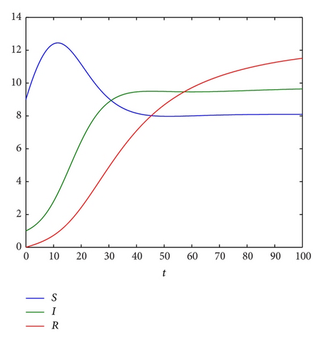
(1) The Endemic Dynamics of the Deterministic Model (1). For the deterministic model (1), R₀ = β₁Λ/μ(μ + α + λ) = 7.407 > 1; thus, it admits a unique endemic equilibrium E^* = (8.1035,9.7664,12.2080) which is globally stable for any initial values (S(0), I(0), R(0)) ∈ Γ according to [10] (see, Figure 1).

Details are in the caption following the image — **Figure 1**
Open in figure viewer PowerPoint

The paths of S(t), I(t), and R(t) for the deterministic model (1) with initial values (S(0), I(0), R(0)) = (9,1, 0). The parameters are taken as (41) (R₀ = 7.407).

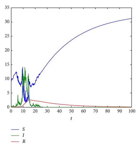
(2) The Stochastic Dynamics of Model (3). For the corresponding stochastic model (3), we choose σ = 0.1; then, we have . Thus, from Theorem 4, we can conclude that for any initial value (S(0), I(0), R(0)) ∈ Γ, disease-free E₀ = (Λ/μ, 0,0) of model (3) is almost surely exponentially stable in Γ (see Figure 2(a)).

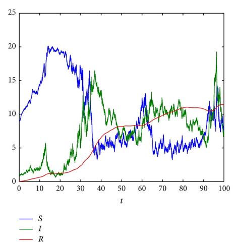
To see the disease dynamics of model (3) more, we decrease the noise intensity σ to be 0.02 and keep the other parameters unchanged. Then, we have . Therefore, the condition of Theorem 4 is not satisfied. In this case, our simulations suggest that model (3) is stochastically persistent (see Figure 2(b)).

5. Concluding Remarks

In this paper, we propose an SIRS epidemic model with media coverage and environment fluctuations to describe disease transmission. It is shown that the magnitude of environmental fluctuations will have an effective impact on the control and spread of infectious diseases. In a nutshell, we summarize our main findings as well as their related biological implications as follows.

Theorem 4 and [10] combined with numerical simulations (see Figures 1 and 2) provide us with a full picture on the dynamics of the deterministic model (1) and stochastic model (3). In [10], the authors showed that the deterministic model (1) admits a unique endemic equilibrium E^* which is globally asymptotically stable if its basic reproduction number R₀ > 1 (see Figure 1). If the magnitude of the intensity of noise σ is large, that is, , the extinction of disease in the stochastic model (3) occurs whether R₀ is greater than 1 or less than 1 (see Figure 2(a)). While the magnitude of the intensity of noise σ is small, one of our most interesting findings is that disease may persist if R₀ > 1, (see Figure 2(b)).

Needless to say, both equilibrium possible approach and parameter possible approach in the present paper have their important roles to play. Obviously, our results in the present paper may be a useful supplement for [10].

Conflict of Interests

The authors declare that there is no conflict of interests regarding the publication of this paper.

Acknowledgments

This research was supported by the National Science Foundation of China (61373005, 11201344, and 11201345) and Zhejiang Provincial Natural Science Foundation (LY12A01014).

References

1 Xiao D. and Ruan S., Global analysis of an epidemic model with nonmonotone incidence rate, Mathematical Biosciences. (2007) 208, no. 2, 419–429, https://doi.org/10.1016/j.mbs.2006.09.025, MR2348123, ZBL1119.92042.
10.1016/j.mbs.2006.09.025
PubMed Web of Science® Google Scholar
2 Cui J.-A., Tao X., and Zhu H., An SIS infection model incorporating media coverage, The Rocky Mountain Journal of Mathematics. (2008) 38, no. 5, 1323–1334, https://doi.org/10.1216/RMJ-2008-38-5-1323, MR2457362, ZBL1170.92024.
10.1216/RMJ-2008-38-5-1323
Web of Science® Google Scholar
3 Cui J., Sun Y., and Zhu H., The impact of media on the control of infectious diseases, Journal of Dynamics and Differential Equations. (2008) 20, no. 1, 31–53, https://doi.org/10.1007/s10884-007-9075-0, MR2385721, ZBL1160.34045.
10.1007/s10884-007-9075-0
PubMed Web of Science® Google Scholar
4 Liu Y. and Cui J.-A., The impact of media coverage on the dynamics of infectious disease, International Journal of Biomathematics. (2008) 1, no. 1, 65–74, https://doi.org/10.1142/S1793524508000023, MR2419647, ZBL1155.92343.
10.1142/S1793524508000023
Web of Science® Google Scholar
5 Li Y. and Cui J., The effect of constant and pulse vaccination on SIS epidemic models incorporating media coverage, Communications in Nonlinear Science and Numerical Simulation. (2009) 14, no. 5, 2353–2365, https://doi.org/10.1016/j.cnsns.2008.06.024, MR2474479, ZBL1221.34034.
10.1016/j.cnsns.2008.06.024
Web of Science® Google Scholar
6 Pang J. and Cui J.-A., An SIRS epidemiological model with nonlinear incidence rate incorporating media coverage, Proceedings of the 2nd International Conference on Information and Computing Science (ICIC ′09), May 2009, 116–119, 2-s2.0-70449561249, https://doi.org/10.1109/ICIC.2009.235.
10.1109/ICIC.2009.235
Google Scholar
7 Brinn M. P., Carson K. V., Esterman A. J., Chang A. B., and Smith B. J., Mass media interventions for preventing smoking in young people, Cochrane Database of Systematic Reviews. (2010) 11, CD001006, 2-s2.0-79952062875.
Google Scholar
8 Funk S., Salathé M., and Jansen V. A. A., Modelling the influence of human behaviour on the spread of infectious diseases: a review, Journal of the Royal Society Interface. (2010) 7, no. 50, 1247–1256, 2-s2.0-77956581464, https://doi.org/10.1098/rsif.2010.0142.
10.1098/rsif.2010.0142
PubMed Web of Science® Google Scholar
9 Xiao Y., Zhao T., and Tang S., Dynamics of an infectious diseases with media/psychology induced non-smooth incidence, Mathematical Biosciences and Engineering. MBE. (2013) 10, no. 2, 445–461, MR3019441, https://doi.org/10.3934/mbe.2013.10.445, ZBL1259.92061.
10.3934/mbe.2013.10.445
PubMed Web of Science® Google Scholar
10 Liu W., A SIRS epidemic model incorporating media coverage with random perturbation, Abstract and Applied Analysis. (2013) 2013, 9, https://doi.org/10.1155/2013/792308, 792308.
10.1155/2013/792308
Google Scholar
11 Young M. E., Norman G. R., and Humphreys K. R., Medicine in the popular press: the influence of the media on perceptions of disease, PLoS ONE. (2008) 3, no. 10, 2-s2.0-56149117102, https://doi.org/10.1371/journal.pone.0003552, e3552.
10.1371/journal.pone.0003552
CAS PubMed Web of Science® Google Scholar
12 Tchuenche J. M. and Bauch C. T., Dynamics of an infectious disease where media coverage influences transmission, ISRN Biomathematics. (2012) 2012, 10, https://doi.org/10.5402/2012/581274, 581274.
10.5402/2012/581274
Google Scholar
13 Spencer S., Stochastic epidemic models for emerging diseases [Ph.D. thesis], 2008, University of Nottingham.
Google Scholar
14 Beddington J. R. and May R. M., Harvesting natural populations in a randomly fluctuating environment, Science. (1977) 197, no. 4302, 463–465, 2-s2.0-0000735971.
10.1126/science.197.4302.463
CAS PubMed Web of Science® Google Scholar
15 Allen L. J. S., An introduction to stochastic epidemic models, Mathematical Epidemiology, 2008, 1945, Springer, Berlin, Germany, 81–130, Lecture Notes in Math., https://doi.org/10.1007/978-3-540-78911-6_3, MR2428373, ZBL1206.92022.
10.1007/978-3-540-78911-6_3
Google Scholar
16 Mao X., Stochastic Differential Equations and Their Applications, 1997, Horwood, Chichester, UK, Horwood Publishing Series in Mathematics & Applications, MR1475218.
Google Scholar
17 Mao X., Marion G., and Renshaw E., Environmental Brownian noise suppresses explosions in population dynamics, Stochastic Processes and their Applications. (2002) 97, no. 1, 95–110, https://doi.org/10.1016/S0304-4149(01)00126-0, MR1870962, ZBL1058.60046.
10.1016/S0304-4149(01)00126-0
Web of Science® Google Scholar
18 Truscott J. E. and Gilligan C. A., Response of a deterministic epidemiological system to a stochastically varying environment, Proceedings of the National Academy of Sciences of the United States of America. (2003) 100, no. 15, 9067–9072, 2-s2.0-0042808451, https://doi.org/10.1073/pnas.1436273100.
10.1073/pnas.1436273100
CAS PubMed Web of Science® Google Scholar
19 Jiang D. and Shi N., A note on nonautonomous logistic equation with random perturbation, Journal of Mathematical Analysis and Applications. (2005) 303, no. 1, 164–172, https://doi.org/10.1016/j.jmaa.2004.08.027, MR2113874, ZBL1076.34062.
10.1016/j.jmaa.2004.08.027
Web of Science® Google Scholar
20 Li X. and Mao X., Population dynamical behavior of non-autonomous Lotka-Volterra competitive system with random perturbation, Discrete and Continuous Dynamical Systems. Series A. (2009) 24, no. 2, 523–545, https://doi.org/10.3934/dcds.2009.24.523, MR2486589, ZBL1161.92048.
10.3934/dcds.2009.24.523
CAS Web of Science® Google Scholar
21 Liu M. and Wang K., Survival analysis of stochastic single-species population models in polluted environments, Ecological Modelling. (2009) 220, no. 9-10, 1347–1357, 2-s2.0-63549091562, https://doi.org/10.1016/j.ecolmodel.2009.03.001.
10.1016/j.ecolmodel.2009.03.001
Web of Science® Google Scholar
22 Ovaskainen O. and Meerson B., Stochastic models of population extinction, Trends in Ecology and Evolution. (2010) 25, no. 11, 643–652, 2-s2.0-77957911001, https://doi.org/10.1016/j.tree.2010.07.009.
10.1016/j.tree.2010.07.009
PubMed Web of Science® Google Scholar
23 Wang W., Cai Y., Wu M., Wang K., and Li Z., Complex dynamics of a reaction-diffusion epidemic model, Nonlinear Analysis: Real World Applications. (2012) 13, no. 5, 2240–2258, https://doi.org/10.1016/j.nonrwa.2012.01.018, MR2911912, ZBL06118775.
10.1016/j.nonrwa.2012.01.018
Web of Science® Google Scholar
24 Ball F. and Neal P., A general model for stochastic SIR epidemics with two levels of mixing, Mathematical Biosciences. (2002) 180, 73–102, John A. Jacquez memorial volumehttps://doi.org/10.1016/S0025-5564(02)00125-6, MR1950749, ZBL1015.92034.
10.1016/S0025-5564(02)00125-6
PubMed Web of Science® Google Scholar
25 Tuckwell H. C. and Williams R. J., Some properties of a simple stochastic epidemic model of SIR type, Mathematical Biosciences. (2007) 208, no. 1, 76–97, https://doi.org/10.1016/j.mbs.2006.09.018, MR2330934, ZBL1116.92061.
10.1016/j.mbs.2006.09.018
PubMed Web of Science® Google Scholar
26 Britton T., Stochastic epidemic models: a survey, Mathematical Biosciences. (2010) 225, no. 1, 24–35, https://doi.org/10.1016/j.mbs.2010.01.006, MR2642269, ZBL1188.92031.
10.1016/j.mbs.2010.01.006
PubMed Web of Science® Google Scholar
27 Gray A., Greenhalgh D., Hu L., Mao X., and Pan J., A stochastic differential equation SIS epidemic model, SIAM Journal on Applied Mathematics. (2011) 71, no. 3, 876–902, https://doi.org/10.1137/10081856X, MR2821582, ZBL1263.34068.
10.1137/10081856X
Web of Science® Google Scholar
28 Yang Q., Jiang D., Shi N., and Ji C., The ergodicity and extinction of stochastically perturbed SIR and SEIR epidemic models with saturated incidence, Journal of Mathematical Analysis and Applications. (2012) 388, no. 1, 248–271, https://doi.org/10.1016/j.jmaa.2011.11.072, MR2869744, ZBL1231.92058.
10.1016/j.jmaa.2011.11.072
Web of Science® Google Scholar
29 Imhof L. and Walcher S., Exclusion and persistence in deterministic and stochastic chemostat models, Journal of Differential Equations. (2005) 217, no. 1, 26–53, https://doi.org/10.1016/j.jde.2005.06.017, MR2170527, ZBL1089.34041.
10.1016/j.jde.2005.06.017
Web of Science® Google Scholar
30 Liu Z., Dynamics of positive solutions to SIR and SEIR epidemic models with saturated incidence rates, Nonlinear Analysis: Real World Applications. (2013) 14, no. 3, 1286–1299, https://doi.org/10.1016/j.nonrwa.2012.09.016, MR3004500, ZBL1261.34040.
10.1016/j.nonrwa.2012.09.016
Web of Science® Google Scholar
31 Mandal P. S. and Banerjee M., Stochastic persistence and stationary distribution in a HollingTanner type preypredator model, Physica A. (2012) 391, no. 4, 1216–1233, 2-s2.0-84655161375, https://doi.org/10.1016/j.physa.2011.10.019.
10.1016/j.physa.2011.10.019
Google Scholar
32 Khasminskii R., Stochastic Stability of Differential Equations, 2012, 66, 2nd edition, Springer, Heidelberg, Germany, Stochastic Modelling and Applied Probability, https://doi.org/10.1007/978-3-642-23280-0, MR2894052.
10.1007/978-3-642-23280-0
Google Scholar
33 Lahrouz A., Omari L., and Kiouach D., Global analysis of a deterministic and stochastic nonlinear SIRS epidemic model, Nonlinear Analysis: Modelling and Control. (2011) 16, no. 1, 59–76, MR2885695, ZBL1271.93015.
10.15388/NA.16.1.14115
Web of Science® Google Scholar
34 Higham D. J., An algorithmic introduction to numerical simulation of stochastic differential equations, SIAM Review. (2001) 43, no. 3, 525–546, https://doi.org/10.1137/S0036144500378302, MR1872387, ZBL0979.65007.
10.1137/S0036144500378302
Web of Science® Google Scholar

Citing Literature

All articles

Stochastic Extinction in an SIRS Epidemic Model Incorporating Media Coverage

Abstract

1. Introduction

2. Model Derivation and Related Definitions

2.1. Model Derivation

2.2. Related Definitions

3. Dynamics of the SDE Model (3)

3.1. Existence of Unique Positive Solution of Model (3)

3.2. Stochastic Extinction of Model (3)

4. Numerical Simulations and Dynamics Comparison

5. Concluding Remarks

Conflict of Interests

Acknowledgments

References

Citing Literature

Figures

References

Information

About Wiley Online Library

Help & Support

Opportunities

Connect with Wiley