Volume 2013, Issue 1 845459

Research Article

Open Access

A Prediction-Correction Dynamic Method for Large-Scale Generalized Eigenvalue Problems

Corresponding Author

Xin-long Luo

[email protected]

orcid.org/0000-0002-4924-6007

School of Information and Communication Engineering, Beijing University of Posts and Telecommunications, P.O. Box 101, Beijing 100876, China bupt.edu.cn

Search for more papers by this author

Jia-ru Lin,

Jia-ru Lin

School of Information and Communication Engineering, Beijing University of Posts and Telecommunications, P.O. Box 101, Beijing 100876, China bupt.edu.cn

Search for more papers by this author

Wei-ling Wu,

Wei-ling Wu

School of Information and Communication Engineering, Beijing University of Posts and Telecommunications, P.O. Box 101, Beijing 100876, China bupt.edu.cn

Search for more papers by this author

Xin-long Luo,

Corresponding Author

Xin-long Luo

[email protected]

orcid.org/0000-0002-4924-6007

School of Information and Communication Engineering, Beijing University of Posts and Telecommunications, P.O. Box 101, Beijing 100876, China bupt.edu.cn

Search for more papers by this author

Jia-ru Lin,

Jia-ru Lin

School of Information and Communication Engineering, Beijing University of Posts and Telecommunications, P.O. Box 101, Beijing 100876, China bupt.edu.cn

Search for more papers by this author

Wei-ling Wu,

Wei-ling Wu

School of Information and Communication Engineering, Beijing University of Posts and Telecommunications, P.O. Box 101, Beijing 100876, China bupt.edu.cn

Search for more papers by this author

First published: 11 September 2013

https://doi.org/10.1155/2013/845459

Citations: 3

Academic Editor: Chang-Hua Lien

Share a link

Email
Wechat
Bluesky

Abstract

This paper gives a new prediction-correction method based on the dynamical system of differential-algebraic equations for the smallest generalized eigenvalue problem. First, the smallest generalized eigenvalue problem is converted into an equivalent-constrained optimization problem. Second, according to the Karush-Kuhn-Tucker conditions of this special equality-constrained problem, a special continuous dynamical system of differential-algebraic equations is obtained. Third, based on the implicit Euler method and an analogous trust-region technique, a prediction-correction method is constructed to follow this system of differential-algebraic equations to compute its steady-state solution. Consequently, the smallest generalized eigenvalue of the original problem is obtained. The local superlinear convergence property for this new algorithm is also established. Finally, in comparison with other methods, some promising numerical experiments are presented.

1. Introduction

In this paper, we consider the smallest generalized eigenvalue problem, which is often encountered in engineering applications such as automatic control, dynamical analysis of structure, electronic structure calculations, and quantum chemistry (see [1, 2] and references therein). For this old and active problem, recently, Gao et al. gave an interesting continuous projected method [3, 4]. This article follows this line and gives a new prediction-correction method based on the dynamical system of differential-algebraic equations (DAEs) for this problem.

First, we convert the smallest eigenvalue problem into an equivalent equality-constrained optimization problem. Second, from the Karush-Kuhn-Tucker conditions of this optimization problem, we obtain a variant of the Rayleigh quotient gradient flow [5, 6], which is formulated by a system of DAEs. Third, applying the implicit Euler method [7], a projected technique [4, 8, 9], and a new time-stepping strategy to that dynamical system of DAEs, we construct a new prediction-correction method to compute a steady-state solution of that special dynamical system. Consequently, we obtain the smallest generalized eigenvalue of (A, B). We also establish the local superlinear convergence property for this new method. Last, in comparison with other methods, some promising numerical experiments are presented. Throughout this article, ∥·∥ denotes the Euclidean vector norm and the corresponding induced matrix norm.

2. Continuous Dynamical Model

The generalized eigenvalue problem (A, B) is to find a scalar λ and nonzero vector x ∈ ℜⁿ to satisfy

()

where A and B are n × n real symmetric matrices and B is positive definite. Problem (1) can be converted to an equivalent equality-constrained optimization problem [4]:

()

If x^* is an optimal solution of problem (2), according to the Karush-Kuhn-Tucker conditions [10, p. 328], then there exists a Lagrange multiplier λ^* such that the following conditions are satisfied at (x^*, λ^*):

()

Therefore, the solution x^* of problem (2) is a generalized eigenvector of (A, B).

Property 1 (Gao et al., 2008 [4]). If x^* is an optimal solution of problem (2) and λ^* is the corresponding Lagrange multiplier, then they satisfy the second-order optimality condition

()

Furthermore, a local minimizer of (2) is also its global minimizer. If x^* is a global minimizer of (2), then it is an eigenvector associated with the smallest generalized eigenvalue of (1).

From the first-order optimality conditions (3) of problem (2), we construct the following negative gradient flow:

()

on the generalized spherical surface,

()

The system of DAEs (5)-(6) is a special dynamical system which is derived from the equality-constrained optimization problem (2). According to the definition of the differential index of DAEs [11], we can verify that the index of DAEs (5)-(6) is two. Therefore, the solution of DAEs (5)-(6) is not easy to be obtained by the general software package such as bdf15s [7, 11, 12]. Thus, we need to devise a special technique for its steady-state solution.

Differentiating the algebraic constraint x^TBx = 1 along the trajectory (x(t), λ(t)) of (5) and (6), we obtain

()

Consequently, we obtain

()

Substituting (8) into (5), we also obtain the following generalized gradient flow:

()

Conversely, if x(t) is a solution of (9), then d(x^TBx)/dt = 0; that is, x(t) satisfies x^TBx = 1, and consequently x(t) also satisfies (5)-(6). Therefore, the continuous dynamical system of (5) and (6) is equivalent to the generalized gradient flow (9).

Since the right-hand-side function of (9) is Lipschitz continuous, it has a unique solution x(t) for any initial point x(0) = x₀. We can verify that the objective function f(x) = x^TAx is monotonically decreasing along the trajectory x(t) of (5)-(6). Actually, from (5)–(8), using the Cauchy-Schwartz inequality |y^Tz | ≤ ∥y∥∥z∥, we have

()

Furthermore, the solution x(t) of (9) converges to an eigenvector x^* associated with the smallest generalized eigenvalue λ^* of (A, B), for almost all initial condition x(0) = x₀, where x₀ satisfies ∥x₀∥ = 1, except for a set of measure zero, that is, the case of a multiple generalized eigenvalue λ^* [5]. Therefore, by following the trajectory x(t) of (5)-(6), we can compute a global minimum point x^* of problem (2), and consequently obtain the smallest generalized eigenvalue λ^* of (A, B).

3. A Prediction-Correction Method

In this section, in order to obtain a steady-state solution of DAEs (5)-(6), we construct a prediction-correction method to follow its trajectory. According to the discussion of Section 2, we know that a steady-state solution of DAEs (5)-(6) is a generalized eigenvector associated with the smallest generalized eigenvalue of (A, B). Therefore, by following the discrete trajectory of DAEs (5)-(6), we can compute an approximate eigenvector associated with the smallest generalized eigenvalue and consequently obtain the smallest generalized eigenvalue.

Note that we mainly consider the steady state of the system of DAEs (5)-(6) and do not care about an accurate solution at its transient-state phase. In order to avoid consuming unnecessary computing time, we adopt the first-order implicit Euler method to follow its trajectory. The time steps of the implicit Euler method are not restricted by the absolute stability property for the linear test equation dx/dt = −μx, where μ > 0 [7], and consequently the implicit Euler method can take large steps at the steady-state phase so that the iteration sequence {x_k} converges rapidly to a stationary point x^* of the system of DAEs (5)-(6).

By applying one implicit Euler iteration to the system of DAEs (5)-(6), we obtain the following iteration formula of the form:

()

where Δt_k is the time step. Note that the system of (11)-(12) is nonlinear, and generally, its solution cannot explicitly be obtained. Therefore, we use the alternating projection idea [13, 14] to handle it.

We replace λ_k+1 with λ_k in (11) to obtain the predicted point

as follows:

()

Since the predicted point

moves away from the elliptic spherical surface, we project this predicted point

onto the unit elliptic spherical surface, so that the iterated point x_k+1 satisfies the algebraic constraint (6); namely, we find the shortest distance between

and the unit elliptic spherical surface. We achieve this aim by solving the following equality-constrained problem:

()

Since the optimal solution of the previously problem is not apparently obtained, we turn to achieve its suboptimal solution. Since matrix B is positive, it can be decomposed as B = L^TL. Let y = Lx. Then, problem (14) is equivalent to the following problem:

()

Since

, we obtain the suboptimal solution by solving the following problem:

()

From the shortest distance between a point and a unit spherical surface being the intersection point of the straight line through the center of that circle and the point and that unit spherical surface, we obtain the previous minimum point as

. Then, the suboptimal solution point of problem (14) is obtained as

()

Now, we use the correction point x_k+1 to update λ_k+1, so that the steady-state equation Ax − λBx = 0 is satisfied as possible. Namely, we find the minimum point of the following problem:

()

Since matrix B is positive, it can be decomposed as B = L^TL. Let z_k+1 = Lx_k+1. Then, the previous minimum problem is equivalent to the following problem:

()

Using the property ∥L^T(L^−TAx_k+1 − λLx_k+1)∥ ≤ ∥L^T∥∥(L^−TAx_k+1 − λLx_k+1)∥, we obtain the suboptimal solution of problem (18) by solving the following problem:

()

It is not difficult to obtain the minimum solution of the previous problem as

()

which is the suboptimal solution of problem (18).

Another issue is how to choose the time step Δt_k at every iteration. We adopt an analogous trust-region technique to adaptively adjust the time step Δt_k. Our intuition is that the time step Δt_k can be enlarged when the predicted point

is also near the elliptic spherical surface x^TBx = 1; otherwise, the time step Δt_k is reduced. In order to measure the distance between

and the unit elliptic spherical surface, we construct the following approximate model:

()

Then,

()

where constants η₁, η₂, γ₁, and γ₂ satisfy

()

According to the previous discussion, we give the following discrete dynamical method for the smallest generalized eigenvalue of (A, B).

Algorithm 1. Prediction-correction method for the smallest generalized eigenvalue.

Step 1. Initialize the parameters. Specify a tolerated error TOL and an initial point x₀ to satisfy

()

Compute

and the residual r₀ = ∥Ax₀ − λ₀Bx₀∥.

Step 2. Repeat for k = 0,1, 2, … until r_k = ∥Ax_k − λ_kBx_k∥ ≤ TOL:

(a)
solve (13) to obtain the predicted point ;
(b)
evaluate (17) to obtain the corrected point x_k+1;
(c)
compute (21) to update the Lagrange multiplier λ_k+1;
(d)
compute the residual
()
(e)
update the time step Δt_k+1 according to the time-stepping scheme (22)-(23);
(f)
accept the trial vector. If ρ_k < η₂, let x_k = x_k+1, λ_k = λ_k+1 and r_k = r_k+1;
(g)
try again starting at (a) with k ← k + 1.

4. Local Convergence Analysis

The sequence (x_k, λ_k) generated by Algorithm 1 follows the continuous trajectory (5)-(6). Adopting the similar estimation technique in [15, 16], we obtain that the local truncation error of x_k is O(Δt_k). According to the standard analysis of numerical ordinary differential equations [7, 11], we know that x_k is close to x(t_k) when Δt_k is small enough in the finite time interval [0, T]. Therefore, we only need to estimate the local convergence rate of x_k in the steady-state phase.

For the convenience of analysis, we decompose matrix B as B = L^TL and denote C = L^−TAL⁻¹. Then, the smallest generalized eigenvalue λ^* of (A, B) and associated with the eigenvector x^* is equivalent to the smallest eigenvalue of symmetric matrix C and associated with the eigenvector y^* = Lx^*, respectively. Therefore, we only need to consider the convergence property of (y_k, λ_k), where y_k = Lx_k. x_k is generated by Algorithm 1.

We denote the error angle between y_k and y^* by ϕ_k = ∠(y_k, y^*). Then, the current iteration y_k can be decomposed as

()

where

and ∥u_k∥ = ∥y^*∥ = 1. From (27), we obtain

()

According to the previous discussion, we give the following local convergence property for Algorithm 1.

Theorem 2. Assume that the sequence (x_k, λ_k) is generated by Algorithm 1. Then, the sequence of error angles ϕ_k tends to zero superlinearly.

Proof. From (21) and Cy^* = λ^*y^*, we have

()

It gives

()

Thus, we choose a small enough positive ε₁ > 0, such as ε₁ = 3/4 | λ^* − μ₂|, and a large enough k to satisfy

()

Then, combining inequality (30), we have

()

Consequently, we obtain

()

We can verify that there exists a positive constant ε_t such that all the time steps Δt_k are bounded below by Δt_min; that is, Δt_k ≥ Δt_min. Actually, from (13), we know that will be close to ∥x_k∥, when Δt_k is small enough. Consequently, for small enough Δt_k, we have

()

According to the time-stepping strategy (23), Δt_k+1 will be enlarged. Therefore, Δt_k are bounded below by a positive number Δt_min.

On the other hand, from (13) and (27), we obtain

()

where u_k+1 = (I + Δt_k(C − λ_kI)) ⁻¹u_k/∥(I + Δt_k(C − λ_kI)) ⁻¹u_k∥ and

. Noticing

and y_k+1 = y^*cos ϕ_k+1 + u_k+1sinϕ_k+1, from (35), we obtain

()

Since u_k is orthogonal to y^* and ∥u_k∥ = 1, u_k can be decomposed as u_k = α₂z₂ + ⋯+α_nz_n, where . Let μ_i (i = 1,2, …, n) be the eigenvalues of C = L^−TAL⁻¹ in ascending order. Thus, from the spectral decomposition of C, for large enough k, we obtain

()

It gives

()

From (36) and (38), for large enough k, we have

()

Combining (33) and (39), we know that ϕ_k converges linearly to zero; namely, y_k converges linearly to y^*, when we choose the initial k such that (y_k, λ_k) is close enough (y^*, λ^*).

Since (y_k, λ_k) converges linearly to (y^*, λ^*), according to the time-stepping strategy (23), we obtain that the time step Δt_k will tend to infinity. Consequently, from inequality (39), we know that ϕ_k superlinearly converges to 0.

Remark 3. From (28) and inequality (39), we have

()

Consequently, the error angles ϕ_k tend to zero cubically, if we adopt a suitable time-stepping strategy such as 1/Δt_k ≈ sin²ϕ_k for large enough k.

Remark 4. The convergence rate of the Rayleigh quotient iteration is cubic; however, its iterate point sequence {x_k} is not guaranteed to converge to the smallest generalized eigenvalue of (A, B) [17]. The convergence rate of Algorithm 1 is less than the convergence rate of the Rayleigh quotient iteration, but the iterate point sequence {x_k} of Algorithm 1 follows the trajectory of the special dynamical system of DAEs (5)-(6), and consequently it converges to a stationary point x^* of the system of DAEs (5)-(6), that is, one of generalized eigenvectors associated with the smallest generalized eigenvalue λ^* of (A, B).

5. Numerical Experiments

We give some numerical experiments for Algorithm 1 (which is denoted by the PCM method), in comparison with the recent continuous projected method by Gao et al. (which is denoted by the GGL method [4]) the restarted Arnoldi method (the EIGS method [18]), and the Jacobi-Davidson method (JDQZ [19, 20]). For Algorithm 1, we pick η₁ = 0.25, η₂ = 0.75, γ₁ = 2, and γ₂ = 0.5 and compute an initial time-step length Δt₀ as follows:

()

For the GGL method, we use the solver ODE45 [12] for the continuous projected dynamical method and set RelTol = 10⁻⁶ and AbsTol = 10⁻⁹, which are suggested in [4]. All of our tests were run in Matlab 2009a environment on a Lenovo Thinkpad laptop X200 with 2.4 GHz processor. The compared methods for the test problems are terminated when the condition

()

is satisfied. The descriptions of test problems and the numerical results are presented by the following.

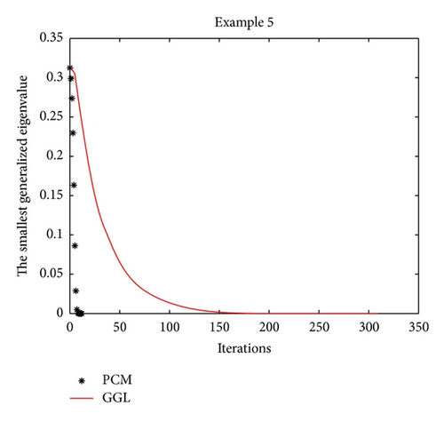
Example 5 (see [4], [21].)This test problem has four generalized eigenvalues. The first three generalized eigenvalues are 0, 0, and 0, and the other is 2. The stiffness and mass matrices are given as follows:

()

It is not difficult to verify that matrix B is positive definite. We choose an initial point x₀ = [0.2,0.6, −0.8,0.6] ^T.

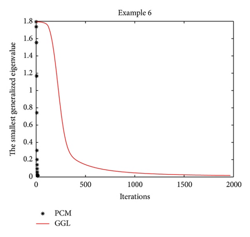
Example 6 (see [4], [21].)The stiffness and mass matrices are given as follows:

()

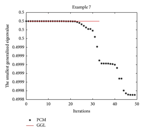
and B = diag (m₁, m₂, …, m_n) with n = 20, k_i = 4 + i, and m_i = 35 − i for i = 1,2, …, 20.

Example 7 (see [22].)This test problem is from fluid flow generalized eigenvalues (see the Bcsstruc1 set in [22]).

Consider the following

()

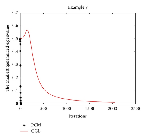
Here, the mass matrix M (bcsstm13.mtx) is a real symmetric positive semidefinite matrix; and the stiffness matrix K (bcsstk13.mtx) is a real positive definite matrix. Therefore, its smallest generalized eigenvalue is zero. In order to test the effect of algorithms, we apply a sift to M as follows:

()

Then, the smallest generalized eigenvalue of (K, B) is 1/2.

Example 8. In order to test the performance of these two methods for large-scale problems, we construct a large-sparse matrix A as follows:

(1)
let A₁ = sparse(diag (ones(n, 1)));
(2)
let A₂ = sparse(diag (ones(n − 1,1), 1));
(3)
let A₃ = sparse(diag (ones(n − 1,1), −1));
(4)
let A = 2A₁ + A₂ + A₃;
(5)
let B = 4A₁ + A₂ + A₃.

Here, sparse.m, diag.m, and ones.m are the Matlab functions, and n is the dimension of A. In our numerical experiments, we set n = 1000 for this test problem.

Numerical results for these four test problems are reported in Table 1. Iter and CPU designate the number of iterations and the computed time (given in seconds), respectively. From the computed results for Examples 5 and 8 in Table 1, we see that the proposed method (the PCM method) manages to find a smaller minimum eigenvalue than the compared method (the GGL method). Furthermore, the computed time of the PCM method is less than the GGL method and the JDQZ method for these test problems. For Example 5, the EIGS method fails since it gives the message: “(A-sigma*B) is singular. The shift is an eigenvalue. Try to use some other shift please,” when we execute it.

Table 1. Comparison with different methods.

Examples		PCM		GGL	EIGS	JDQZ
Examples	λ_k	Iter (CPU)	λ_k	Iter (CPU)	CPU	CPU
Example 5	1.0e − 13	12 (0.021)	4.5e − 11	77 (0.178)	FAIL	FAIL
Example 6	0.01337	18 (0.004)	0.01344	3389 (0.36)	0.01	0.49
Example 7	0.4998	49 (2.556)	0.5	33 (6.643)	0.24	14.17
Example 8	1.1e − 5	28 (0.024)	0.0122	514 (169.3)	0.02	0.686

In order to record the convergence history, we draw the iteration trajectory of the smallest eigenvalue computed by the PCM method and by the GGL method for every test problem in Figures 1, 2, 3, and 4. From those figures, we find that Algorithm 1 (the PCM method) achieves the steady state of the dynamical system faster than the GGL method.

Details are in the caption following the image — **Figure 1**
Open in figure viewer PowerPoint

Numerical results of Example 5 with PCM and GGL methods.

In order to test the sensitivity of Algorithm 1, we compute the test problems with Algorithm 1 for different parameters γ₁, γ₂, η₁, and η₂. The robustness of Algorithm 1 is mainly determined by the parameters η₁ and η₂ and the parameters η₁ and η₂ affect its efficiency. Thus, we fix parameters γ₁ = 2 and γ₂ = 1/2. We choose four groups of parameters η₁ and η₂ as following:

(I)
η₁ = 0.25, η₂ = 0.75;
(II)
η₁ = 0.1, η₂ = 0.9;
(III)
η₁ = 0.3, η₂ = 0.7;
(IV)
η₁ = 0.4, η₂ = 0.8.

The numerical results are reported in Table 2. From Table 2, we find that Algorithm 1 is not sensitive for different parameters η₁ around 0.25 and η₂ around 0.75. Thus, we set the default parameters η₁ = 0.25 and η₂ = 0.75 in Algorithm 1.

Table 2. Numerical results for different parameters of Algorithm 1.

Examples	(I)	(II)	(III)	(IV)
Examples	Iter (CPU)	Iter (CPU)	Iter (CPU)	Iter (CPU)
Example 5	12	12	12	12
Example 6	19	19	19	17
Example 7	49	49	50	45
Example 8	26	31	22	22

6. Conclusions

This paper discusses the connection between the smallest generalized eigenvalue problem and the continuous dynamical system of DAEs. The trajectory of this special dynamical system is followed by a new prediction-correction method (Algorithm 1), which is derived from the implicit Euler formula and an analogous trust-region technique. Consequently, an equilibrium point x^* of this continuous dynamical system is obtained. This equilibrium point x^* is also a generalized eigenvector associated with the smallest generalized eigenvalue. The local superlinear property for the new prediction-correction method is presented. Numerical experiments indicate that Algorithm 1 is promising for the smallest generalized eigenvalue problem. Another interesting issue is whether or not the second-order, pseudo-transient method [23] obtains the superior numerical property for this special dynamical system of DAEs (5)-(6). We would like to consider this issue in our future works.

Acknowledgments

Xin-long Luo is grateful to Proffessor Li-Zhi Liao for fruitful discussions when he visited Hong Kong Baptist University in winter, 2011. This work was supported in part by Grant 2009CB320401 from the National Basic Research Program of China, Grant YBWL2011085 from Huawei Technologies Co., Ltd., and Grant YJCB2011003HI from the Innovation Research Program of Huawei Technologies Co., Ltd., Grant BUPT2009RC0118 from the Fundamental Research Funds for the Central Universities.

References

1 Auckenthaler T., Auckenthaler T., Bungartz H.-J. et al., Parallel solution of partial symmetric eigenvalue problems from electronic structure calculations, Parallel Computing. (2011) 37, no. 11, 783–794, https://doi.org/10.1016/j.parco.2011.05.002.
10.1016/j.parco.2011.05.002
Web of Science® Google Scholar
2 Saad Y., Numerical Methods for Large Eigenvalue Problems, 1992, Manchester University Press, Manchester, England, Algorithms and Architectures for Advanced Scientific Computing, MR1177405.
Google Scholar
3 Golub G. H. and Liao L.-Z., Continuous methods for extreme and interior eigenvalue problems, Linear Algebra and its Applications. (2006) 415, no. 1, 31–51, https://doi.org/10.1016/j.laa.2005.01.009, MR2214745, ZBL1092.65029.
10.1016/j.laa.2005.01.009
Web of Science® Google Scholar
4 Gao X.-B., Golub G. H., and Liao L.-Z., Continuous methods for symmetric generalized eigenvalue problems, Linear Algebra and its Applications. (2008) 428, no. 2-3, 676–696, https://doi.org/10.1016/j.laa.2007.08.034, MR2374572, ZBL1140.65029.
10.1016/j.laa.2007.08.034
Web of Science® Google Scholar
5 Helmke U. and Moore J. B., Optimization and Dynamical Systems, 1996, 2nd edition, Springer.
Google Scholar
6 Mahony R. and Absil P.-A., The continuous-time Rayleigh quotient flow on the sphere, Linear Algebra and its Applications. (2003) 368, 343–357, https://doi.org/10.1016/S0024-3795(02)00730-9, MR1983213, ZBL1030.65025.
10.1016/S0024-3795(02)00730-9
Web of Science® Google Scholar
7 Gear C. W., Numerical Initial Value Problems in Ordinary Differential Equations, 1971, Prentice-Hall, Englewood Cliffs, NJ, USA, MR0315898.
Google Scholar
8 He B., Yuan X., and Zhang J. J. Z., Comparison of two kinds of prediction-correction methods for monotone variational inequalities, Computational Optimization and Applications. (2004) 27, no. 3, 247–267, https://doi.org/10.1023/B:COAP.0000013058.17185.90, MR2035715, ZBL1061.90111.
10.1023/B:COAP.0000013058.17185.90
Web of Science® Google Scholar
9 He B. and Yuan X., On the O(1/n) convergence rate of the Douglas-Rachford alternating direction method, SIAM Journal on Numerical Analysis. (2012) 50, no. 2, 700–709, https://doi.org/10.1137/110836936, MR2914282, ZBL1245.90084.
10.1137/110836936
Web of Science® Google Scholar
10 Nocedal J. and Wright S. J., Numerical Optimization, 1999, Springer, New York, NY, USA, Springer Series in Operations Research, https://doi.org/10.1007/b98874, MR1713114.
10.1007/b98874
Web of Science® Google Scholar
11 Ascher U. M. and Petzold L. R., Computer Methods for Ordinary Differential Equations and Differential-Algebraic Equations, 1998, Society for Industrial and Applied Mathematics, Philadelphia, Pa, USA, https://doi.org/10.1137/1.9781611971392, MR1638643, ZBL1089.01501.
10.1137/1.9781611971392
Google Scholar
12 Shampine L. F. and Reichelt M. W., The Matlab ODE suite, SIAM Journal on Scientific Computing. (1997) 18, no. 1, 1–22, https://doi.org/10.1137/S1064827594276424, MR1433374, ZBL0868.65040.
10.1137/S1064827594276424
Web of Science® Google Scholar
13 Liu S.-T. and Luo X.-L., A method based on Rayleigh quotient gradient flow for extreme and interior eigenvalue problems, Linear Algebra and its Applications. (2010) 432, no. 7, 1851–1863, https://doi.org/10.1016/j.laa.2009.12.023, MR2592921, ZBL1186.65043.
10.1016/j.laa.2009.12.023
Web of Science® Google Scholar
14 Ng M. K., Wang F., and Yuan X., Inexact alternating direction methods for image recovery, SIAM Journal on Scientific Computing. (2011) 33, no. 4, 1643–1668, https://doi.org/10.1137/100807697, MR2821262, ZBL1234.94013.
10.1137/100807697
Web of Science® Google Scholar
15 Kelley C. T., Liao L.-Z., Qi L., Chu M. T., Reese J. P., and Winton C., Projected pseudotransient continuation, SIAM Journal on Numerical Analysis. (2008) 46, no. 6, 3071–3083, https://doi.org/10.1137/07069866X, MR2439502, ZBL1180.65060.
10.1137/07069866X
Web of Science® Google Scholar
16 Luo X. L., A dynamical method of DAEs for the smallest eigenvalue problem, Journal of Computational Science. (2012) 3, no. 3, 113–119, https://doi.org/10.1016/j.jocs.2012.01.002.
10.1016/j.jocs.2012.01.002
Web of Science® Google Scholar
17 Parlett B. N., The Symmetric Eigenvalue Problem, 1998, Society for Industrial and Applied Mathematics, Philadelphia, Pa, USA, Classics in Applied Mathematics, Corrected reprint of the 1980 originalhttps://doi.org/10.1137/1.9781611971163, MR1490034.
10.1137/1.9781611971163
Google Scholar
18 MATLAB R2009a, http://www.mathworks.com.
Google Scholar
19 Fokkema D. R., Sleijpen G. L. G., and Van der Vorst H. A., Jacobi-Davidson style QR and QZ algorithms for the reduction of matrix pencils, SIAM Journal on Scientific Computing. (1998) 20, no. 1, 94–125, https://doi.org/10.1137/S1064827596300073, MR1639102.
10.1137/S1064827596300073
Web of Science® Google Scholar
20 http://www.staff.science.uu.nl/?sleij101/index.html.
Google Scholar
21 Zhang T., Law K. H., and Golub G. H., On the homotopy method for perturbed symmetric generalized eigenvalue problems, SIAM Journal on Scientific Computing. (1998) 19, no. 5, 1625–1645, https://doi.org/10.1137/S1064827596299755, MR1618745, ZBL0917.65035.
10.1137/S1064827596299755
Web of Science® Google Scholar
22 Matrix Market, http://math.nist.gov/MatrixMarket.
Google Scholar
23 Luo X.-l., A second-order pseudo-transient method for steady-state problems, Applied Mathematics and Computation. (2010) 216, no. 6, 1752–1762, https://doi.org/10.1016/j.amc.2009.12.029, MR2645309, ZBL1197.65050.
10.1016/j.amc.2009.12.029
Web of Science® Google Scholar

All articles

A Prediction-Correction Dynamic Method for Large-Scale Generalized Eigenvalue Problems

Abstract

1. Introduction

2. Continuous Dynamical Model

3. A Prediction-Correction Method

4. Local Convergence Analysis

5. Numerical Experiments

6. Conclusions

Acknowledgments

References

Figures

References

Information

About Wiley Online Library

Help & Support

Opportunities

Connect with Wiley

A Prediction-Correction Dynamic Method for Large-Scale Generalized Eigenvalue Problems

Abstract

1. Introduction

2. Continuous Dynamical Model

3. A Prediction-Correction Method

4. Local Convergence Analysis

5. Numerical Experiments

6. Conclusions

Acknowledgments

References

Figures

References

Related

Information