An explicit multistep mixed finite element method is proposed and discussed for regularized long wave (RLW) equation. The spatial direction is approximated by the mixed Galerkin method using mixed linear space finite elements, and the time direction is discretized by the explicit multistep method. The optimal error estimates in L² and H¹ norms for the scalar unknown u and its flux q = u_x based on time explicit multistep method are derived. Some numerical results are given to verify our theoretical analysis and illustrate the efficiency of our method.

1. Introduction

In this paper, we consider the following initial boundary problem of RLW equation:

(1)

where I = (a, b) is a bounded open interval, J = (0, T] with 0 < T < ∞. The initial value u₀(x) is given function, and the coefficients β, γ, δ are all positive constants.

In recent years, large nonlinear phenomena are found in many research fields, for example, physics, biology, fluid dynamics, and so forth. These phenomena can be described by the mathematical model of some nonlinear evolution equations. In particular, some attention has also been paid to nonlinear RLW equations [1, 2] which play a very important role in the study of nonlinear dispersive waves. Solitary waves are wave packet or pulses, which propagate in nonlinear dispersive media. Due to dynamical balance between the nonlinear and dispersive effects, these waves retain an unchanged waveform. A soliton is a very special type of solitary wave, which also keeps its waveform after collision with other solitons. The regularized long wave (RLW) equation is an alternative description of nonlinear dispersive waves to the more usual Korteweg-de Vries (KdV) equation. Mathematical theories and numerical methods for (1) were considered in [1–24]. The existence and uniqueness of the solution of RLW equation are discussed in [5]. Their analytical solutions were found under restricted initial and boundary conditions, and therefore they got interest from a numerical point of view. Several numerical methods for the solution of the RLW equation have been introduced in the literature. These include a variety of difference methods [5–8, 17], finite element methods based on Galerkin and collocation principles [9–13], mixed finite element methods [14–16], meshfree method [18], adomian decomposition method [19], and so on.

In [25], Chatzipantelidis studied the explicit multistep methods for some nonlinear partial differential equations and discussed some mathematical theories. Akrivis et al. [26] studied the multistep method for some nonlinear evolution equations. Mei and Chen [20] presented the explicit multistep method based on Galerkin method for regularized long wave (RLW) equation. In this paper, our purpose is to propose and study an explicit multistep mixed method, which combines a mixed Galerkin method in the spatial direction and the explicit multistep method in the time direction, for RLW equation. We derive optimal error estimates in L² and H¹ norms for the scalar unknown u and its flux q = u_x for the fully discrete explicit multistep mixed scheme and compare our method’s accuracy with some other numerical schemes. Compared to the numerical methods in [20, 25, 26], we not only obtain the approximation solution for u, but also get the approximation solution for q = u_x.

The layout of the paper is as follows. In Section 2, an explicit multistep mixed scheme and numerical process are given. The optimal error estimates in L² and H¹ norms for the scalar unknown u and its flux q = u_x for the fully discrete explicit multistep mixed scheme are proved in Section 3. In Section 4, some numerical results are shown to confirm our theoretical analysis. Finally, some concluding remarks are given in Section 5. Throughout this paper, C will denote a generic positive constant which does not depend on the spatial mesh parameter h or time discretization parameter Δt.

2. The Mixed Numerical Scheme

With the auxiliary variable q = u_x, we reformulate (1) as the following first-order coupled system:

(2)

We consider the following mixed weak formulation of (2). Find

satisfying:

(3)

(4)

Noting the Dirichlet boundary conditions u_t(a, t) = u_t(b, t) = 0 and q_t = u_xt, we can get (u_t, −w_x) = (u_xt, w) = (q_t, w) easily and then get the scheme (4).

Let V_h and W_h be finite dimensional subspaces of

and H¹, respectively, defined by

(5)

where T_h is a partition of

into N subintervals I_j = [x_j, x_j+1], j = 0,1, 2, …, (N − 1), h_j = h_j+1 − h_j, h = max _{0≤j≤N−1}h_j, and P_m(I_j) denotes the polynomials of degree less than or equal to m in I_j.

The semidiscrete mixed finite element method for (3) and (4) consists in determining {u^h, q^h}:[0, T] ↦ V_h × W_h such that

(6)

(7)

In the following discussion, we will give an explicit multistep mixed scheme. We take linear finite element spaces V_h = span {φ₀, φ₁, …, φ_N} and W_h = span {φ₀, φ₁, …, φ_N}, and then u_h and q_h can be expressed as the following formulation:

(8)

Substitute (8) into (6) and (7), and take v^h = φ_j and w^h = φ_j in (6) and (7), respectively, to obtain

(9)

where j = 0,1, 2, …, N.

We subdivide the space variable domain [a, b] into uniform subintervals with N + 1 grid points x_k, k = 0, …, N, such that a = x₀ < x₁ < ⋯<x_N = b, h = x_k+1 − x_k = (b − a)/N. Using the local coordinate transformation x = x_k + μh, 0 ≤ μ ≤ 1, we transform a subinterval [x_k, x_k+1] into a standard interval [0,1]. Furthemore, we have

(10)

We take linear basis functions defined as follows:

(11)

and then the variables u and q over the element [x_k, x_k+1] are written as

(12)

Then, we get the following equations:

(13)

Then, the system (13) has the following matrix form:

(14)

with the following element matrices:

(15)

Assembling contributions from all elements, we obtain the following coupled system of nonlinear matrix equations:

(16)

To formulate a fully discrete scheme, we consider a uniform partition of

with time step length Δt = T/N, N ∈ Z⁺, and time levels tⁿ = nΔt, n = 0, …, N. We now discuss a fully discrete scheme based on a linear explicit multistep method. We now define Uⁿ ∈ V_h and Zⁿ ∈ W_h as approximations to u(tⁿ) and q(t_n), respectively, and formulate the following fully discrete linear explicit multistep mixed scheme:

(17)

with given the initial approximations U⁰, …, U^p−1 and Z⁰, …, Z^p−1. In the explicit multistep mixed system (17), the parameter variable α_i and σ_i is described by the coefficients of the term χⁱ, for the following polynomials α(χ) and σ(χ), respectively:

(18)

In this paper, we consider the explicit 2-step mixed method for the RLW equation. For p = 2, we obtained easily

(19)

Substituting (19) into (17), we obtain the following 2-step mixed scheme:

(20)

Remark 1. There have been many numerical schemes for the RLW equation, but we have not seen the related research on explicit multistep mixed element method for RLW equation in the literature. From the viewpoint of numerical theory, we propose a mixed element scheme (6) and (7), which is different from some other mixed finite element methods in [14–16], for the RLW equation and derive some a priori error estimates based on the explicit multistep mixed element method. From the perspective of numerical calculation, our method is efficient for RLW equation.

3. Two-Step Mixed Scheme and Optimal Error Estimates

3.1. Two-Step Mixed Scheme and Some Lemmas

In this section, we will discuss some a priori error estimates based on explicit 2-step mixed finite element method for the RLW equation. For the fully discrete procedure, let 0 = t₀ < t₁ < ⋯<t_N = T be a given partition of the time interval [0, T] with step length Δt = T/N, for some positive integer N. For a smooth function ϕ on [0, T], define ϕⁿ = ϕ(t_n).

The system (3) and (4) has the following formulation at t = t_n+1:

(21)

Based on system (17), we get an equivalent formulation for system (21) as

(22)

(23)

where

(24)

We now find a pair {Uⁿ⁺¹, Zⁿ⁺¹} in V_h × W_h satisfying

(25)

(26)

For the theoretical analysis of a priori error estimates, we define the following projections.

Lemma 2 (see [15], [27], [28].)One defines the elliptic projection by

(27)

With

, the following estimates are well known for j = 0,1:

(28)

Lemma 3 (see [15], [27], [28].)Furthermore, one also defines a Ritz projection of q as the solution of

(29)

where A(q, w) = (q_x, w_x) + λ(q, w), and λ is taken appropriately so that

(30)

where μ₀ is a positive constant. Moreover, it is easy to verify that A(·, ·) is bounded.

With , the following estimates hold:

(31)

For fully discrete error estimates, we now write the errors as

(32)

Combine (27), (29), (22), (23), (25), and (26) at t = t_n+1 to get the following error equations:

(33)

(34)

where

(35)

Lemma 4. For τⁿ⁺¹, , , and , the following estimates hold:

(36)

Proof. Using the Taylor expansion, we have

(37)

(38)

Combining (37) and (38) and noting that −2Δt = 2(t_n − t_n+1) = t_n−1 − t_n+1, we obtain

(39)

From (39), we have

(40)

Using a similar estimate as the one for

, we have

(41)

where t_n < t_Δ3 < t_n+1, t_n−1 < t_Δ4 < t_n+1.

From (41), we have

(42)

Using the Taylor expansion and noting that −2Δt = 2(t_n − t_n+1) = t_n−1 − t_n+1, we have

(43)

Using (43), we obtain

(44)

By (44), we have

(45)

Using the similar method to the estimate for ∥τⁿ⁺¹∥ and (31), we obtain

(46)

3.2. Optimal Error Estimates

In this subsection, we derive the fully discrete optimal error estimates and obtain the following theorem.

Theorem 5. Assuming that U⁰, U¹ ∈ V_h and Z⁰, Z¹ ∈ W_h are given, then for 1 ≤ J ≤ M, j = 0,1, one has

(47)

Proof. Taking v^h = ςⁿ⁺¹ in (33) and using Cauchy-Schwarz’s inequality and Poincaré’s inequality, we get

(48)

Set w^h = ξⁿ⁺¹ in (34) to obtain

(49)

Use (48) as well as the Cauchy-Schwarz and Young’s inequalities to obtain

(50)

Note that

(51)

(52)

We now estimate T₁, T₂, T₃, and T₄ as

(53)

Substituting (53) into (52), we obtain

(54)

Substituting (36), (51), and (54) into (50), using (48), and summing from n = 1,2, …, J, the resulting inequality becomes

(55)

Choose Δt₀ in such a way that for 0 < Δt ≤ Δt₀, (1 − CΔt) > 0. Then, as an application of Gronwall’s lemma, we obtain

(56)

Combine (28), (31), and (56) with the triangle inequality to complete the L² and H¹ error estimates for q. Furthermore, use (48) and the triangle inequality to complete the optimal error estimates for ∥u(t_n) − Uⁿ∥ and

Remark 6. Compared to a variety of difference methods in [17], our method is studied based on mixed element scheme (6) and (7).

Remark 7. Although some convergence proofs of multistep methods for RLW/BBM are provided in [20, 25, 29], our convergence results of multistep methods are proved based on a mixed finite element scheme. Based on the current discussion, we have to provide the detailed proofs for multistep mixed finite element methods in this paper.

4. Numerical Results

In order to test the viability of the proposed method, we consider a test problem. We write conservation laws as [3, 4]

(57)

where Q₁, Q₂, and Q₃ are usually called mass, momentum, and energy, respectively, which are observed to check the conservation of the numerical scheme.

We consider RLW equation (1) and let, in (1), δ = γ = β = 1. Then, the solitary wave solution of (1) is

(58)

where

(59)

We consider the motion of a single solitary wave and take as initial condition, with c = 0.1 and x₀ = 0,

(60)

The corresponding exact solution with initial condition (60) is

(61)

In this procedure, we take space-time domain as −40 ≤ x ≤ 60 and 0 ≤ t ≤ 20.

In Table 1, we take spatial mesh parameter h = 0.125 and time discretization parameter Δt = 0.1 and list the three invariants Q₁, Q₂, and Q₃ and the optimal error estimate in L² and L^∞ norms for u at different times t = 0, 4, 8, 12, 16, and 20. At the same time, we show some numerical results at time t = 20 obtained by other numerical methods in Table 1. From Table 1, we find that our method is more accurate than the numerical methods in [17, 18, 28] but is less than the numerical methods in [23, 24]. From the shown results in Table 1, we can see that Q₁, Q₂ and Q₃ keep almost constants, so the conservation for our method is very well.

Table 1. Solitary wave Amp. 0.3 and the errors in L² and L^∞ norms for u, Q₁, Q₂, and Q₃ at t = 20, h = 0.125, Δt = 0.1, and −40 ≤ x ≤ 60.

Method	Time	Q₁	Q₂	Q₃	L² for u	L^∞ for u
Our method	0	3.9797	0.8104	2.5787	0	0
	4	3.9797	0.8104	2.5786	3.6304e − 004	5.2892e − 005
	8	3.9797	0.8104	2.5786	7.2873e − 004	5.8664e − 005
	12	3.9797	0.8104	2.5787	1.0817e − 003	6.3283e − 005
	16	3.9795	0.8104	2.5787	1.4186e − 003	6.8001e − 005
	20	3.9790	0.8103	2.5785	1.7396e − 003	7.7154e − 005
[20]	20	3.9800	0.8104	2.5792	1.7569e − 003	6.8432e − 004
[21]	20	3.9820	0.8087	2.5730	4.688e − 003	1.755e − 003
[22]	20	3.9905	0.8235	2.6740	2.157e − 003	—
[23]	20	3.9616	0.8042	2.5583	0.018e − 003	1.566e − 003
[24]	20	3.9821	0.8112	2.5813	0.511e − 003	0.198e − 003

In Tables 2 and 3, we take spatial mesh parameter h = 0.125 and obtain the optimal error results in L² and L^∞ norms for u at different times t = 0, 4, 8, 12, 16, and 20 with different time discretization parameters Δt = 0.1,0.2, and 0.4. From Tables 2 and 3, we see easily that the convergence rate for time is close to order 2. Similarly, the results for q are shown in Tables 4 and 5.

Table 2. Convergence order and error in L² norm for u of time with h = 0.125 and c = 0.1.

Time	Δt = 0.4	Δt = 0.2	Δt = 0.1	Order (0.2/0.4)	Order (0.1/0.2)
4	5.3805e − 003	1.4267e − 003	3.6304e − 004	1.9151	1.9745
8	1.1688e − 002	2.9411e − 003	7.2873e − 004	1.9906	2.0129
12	1.7830e − 002	4.3997e − 003	1.0817e − 003	2.0188	2.0241
16	2.3751e − 002	5.7916e − 003	1.4186e − 003	2.0360	2.0295
20	2.9434e − 002	7.1148e − 003	1.7396e − 003	2.0486	2.0321

Table 3. Convergence order and error in L^∞ norm for u of time with h = 0.125 and c = 0.1.

Time	Δt = 0.4	Δt = 0.2	Δt = 0.1	Order (0.2/0.4)	Order (0.1/0.2)
4	8.0743e − 004	2.0299e − 004	5.2892e − 005	1.9919	1.9403
8	9.1778e − 004	2.2908e − 004	5.8664e − 005	2.0023	1.9653
12	9.9866e − 004	2.4966e − 004	6.3283e − 005	2.0000	1.9801
16	1.0718e − 003	2.6685e − 004	6.8001e − 005	2.0059	1.9724
20	1.1277e − 003	2.8609e − 004	7.7154e − 005	1.9788	1.8907

Table 4. Convergence order and error in L² norm for q of time with h = 0.125 and c = 0.1.

Time	Δt = 0.4	Δt = 0.2	Δt = 0.1	Order (0.2/0.4)	Order (0.1/0.2)
4	2.4430e − 003	6.4427e − 004	1.6260e − 004	1.9229	1.9863
8	5.1823e − 003	1.2934e − 003	3.1976e − 004	2.0024	2.0161
12	7.6616e − 003	1.8713e − 003	4.5963e − 004	2.0336	2.0255
16	9.8719e − 003	2.3787e − 003	5.8232e − 004	2.0532	2.0303
20	1.1843e − 002	2.8251e − 003	6.8991e − 004	2.0677	2.0338

Table 5. Convergence order and error in L^∞ norm for q of time with h = 0.125 and c = 0.1.

Time	Δt = 0.4	Δt = 0.2	Δt = 0.1	Order (0.2/0.4)	Order (0.1/0.2)
4	1.1595e − 004	2.7265e − 005	6.3127e − 006	2.0884	2.1107
8	1.9712e − 004	4.6625e − 005	1.0725e − 005	2.0799	2.1201
12	2.5295e − 004	5.9837e − 005	1.3579e − 005	2.0797	2.1397
16	2.9012e − 004	6.8641e − 005	1.5594e − 005	2.0795	2.1381
20	3.1768e − 004	7.5864e − 005	1.7195e − 005	2.0661	2.1414

In Tables 6 and 7, the optimal error results in L² and L^∞ norms for u at different times t = 0, 4, 8, 12, 16, and 20 with different spatial mesh parameters h = 0.2, 0.4, and 0.8 and time discretization parameter Δt = 0.01 are shown. It is easy to see that the convergence rate for space is close to order 2. The similar results for q are listed in Tables 8 and 9.

Table 6. Convergence order and error in L² norm for u of space with Δt = 0.01 and c = 0.1.

Time	h = 0.8	h = 0.4	h = 0.2	Order (0.4/0.8)	Order (0.2/0.4)
4	1.7109e − 003	4.2677e − 004	1.1449e − 004	1.9940	1.8982
8	1.8945e − 003	4.6862e − 004	1.1924e − 004	2.0195	1.9746
12	2.1232e − 003	5.2130e − 004	1.3025e − 004	2.0102	2.0008
16	2.3559e − 003	5.7598e − 004	1.4421e − 004	2.0589	1.9978
20	2.5778e − 003	6.3407e − 004	1.7877e − 004	2.0358	1.8265

Table 7. Convergence order and error in L^∞ norm for u of space with Δt = 0.01 and c = 0.1.

Time	h = 0.8	h = 0.4	h = 0.2	Order (0.4/0.8)	Order (0.2/0.4)
4	2.1763e − 003	5.8447e − 004	1.5502e − 004	1.8967	1.9147
8	4.7892e − 003	1.2098e − 003	3.0533e − 004	1.9850	1.9863
12	7.2371e − 003	1.7871e − 003	4.4434e − 004	2.0178	2.0079
16	9.4746e − 003	2.3084e − 003	5.7081e − 004	2.0372	2.0158
20	1.1534e − 002	2.7859e − 003	6.8980e − 004	2.0497	2.0139

Table 8. Convergence order and error in L² norm for q of space with Δt = 0.01 and c = 0.1.

Time	h = 0.8	h = 0.4	h = 0.2	Order (0.4/0.8)	Order (0.2/0.4)
4	2.3426e − 004	5.4759e − 005	1.2581e − 005	2.0969	2.1218
8	4.2831e − 004	1.0038e − 004	2.2853e − 005	2.0932	2.1350
12	5.7270e − 004	1.3452e − 004	3.0443e − 005	2.0900	2.1436
16	6.7812e − 004	1.5951e − 004	3.5927e − 005	2.0879	2.1505
20	7.5693e − 004	1.7832e − 004	4.0176e − 005	2.0857	2.1501

Table 9. Convergence order and error in L^∞ norm for q of space with Δt = 0.01 and c = 0.1.

Time	h = 0.8	h = 0.4	h = 0.2	Order (0.4/0.8)	Order (0.2/0.4)
4	1.1957e − 003	3.1367e − 004	7.8812e − 005	1.9305	1.9928
8	2.4344e − 003	6.0206e − 004	1.4825e − 004	2.0156	2.0219
12	3.4768e − 003	8.3962e − 004	2.0540e − 004	2.0500	2.0313
16	4.3743e − 003	1.0402e − 003	2.5371e − 004	2.0722	2.0356
20	5.1677e − 003	1.2153e − 003	2.9544e − 004	2.0882	2.0404

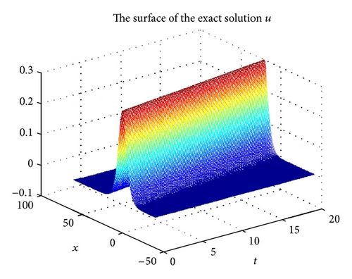
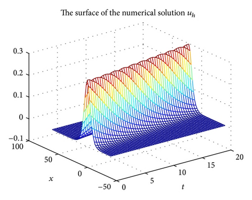
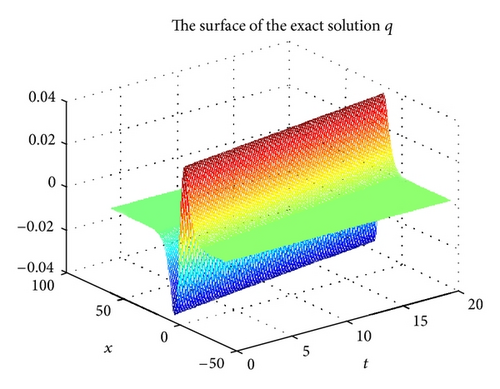
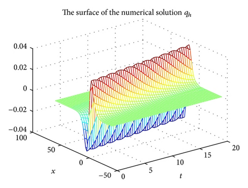
Figure 1 shows the surface for the exact solution u in space-time domain ((x, t)∈[−20,60]×[0,20]), and the corresponding surface for the numerical solution u_h with h = 2 and Δt = 0.4 is described in Figure 2. From Figures 1 and 2, we see easily that the exact solution u is approximated very well by the numerical solution u_h. In Figures 3 and 4, we show the surface for the exact solution q and the numerical solution q_h, respectively, with h = 2 and Δt = 0.4 and obtain a good approximation solution q_h for the exact solution q.

Details are in the caption following the image — **Figure 1**
Open in figure viewer PowerPoint

Surface for exact solution u.

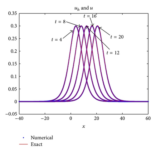
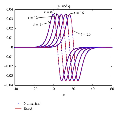
The comparison between the exact solution u and the numerical solution u_h is described at different times t = 4,8, 12,16, and 20 with h = 0.125 and Δt = 0.2 in Figure 5. The similar comparison for the exact solution q and the numerical solution q_h is shown in Figure 6. Figures 5 and 6 show that the solitary wave for u and q moves to the right with unchanged form and velocity, respectively. Furthermore, the exact solutions u and q are approximated well by the numerical solutions u_h and q_h, respectively.

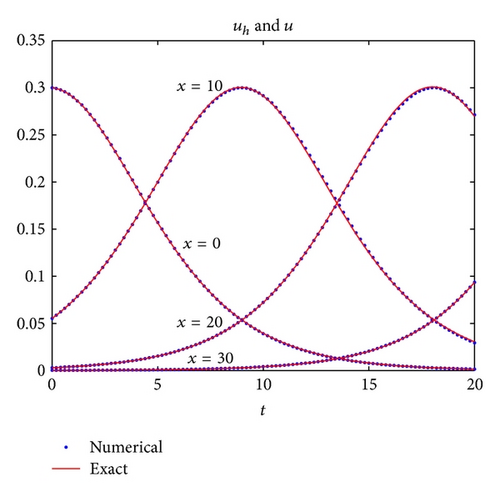
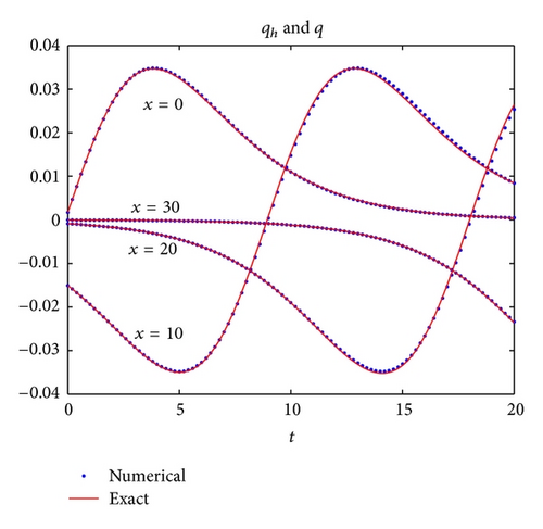
In Figure 7, we show the comparison between u and u_h at different spaces x = 0,10,20, and 30 with h = 0.125 and Δt = 0.2 to verify the efficiency for the proposed scheme in this paper. Figure 8 describes a similar result for q.

From the previous analysis in Tables 1–9 and Figures 1–8, we can see that the numerical results confirm the theoretical results of Theorem 5 and our method is efficient for RLW equation.

5. Concluding Remarks

In this paper, we propose and analyze an explicit multistep mixed finite element method, which combines spatial mixed finite element method and time explicit multistep method, for RLW equation. We discuss the numerical process for our method, prove the theoretical results for the fully discrete explicit multistep mixed scheme, obtain the optimal convergence order, and compare our method’s accuracy with some other numerical schemes. Compared with the numerical method in [20, 25, 26], our method can obtain the optimal error estimates in L² and H¹ norms for the scalar unknown u and its flux q = u_x simultaneously. From our numerical results, we can see that our method is efficient for RLW equation.

Acknowledgments

This work was supported by the National Natural Science Fund of China (11061021), the Scientific Research Projection of Higher Schools of Inner Mongolia (NJZZ12011 and NJZY13199), the Natural Science Fund of Inner Mongolia Province (2012MS0108 and 2012MS0106), and the Program of Higher-Level Talents of Inner Mongolia University (125119).

References

1 Peregrine D. H., Calculations of the development of an undular bore, Journal of Fluid Mechanics. (1966) 25, no. 2, 321–330.
10.1017/S0022112066001678
Web of Science® Google Scholar
2 Benjamin T. B., Bona J. L., and Mahony J. J., Model equations for long waves in nonlinear dispersive systems, Philosophical Transactions of the Royal Society of London A. (1972) 272, no. 1220, 47–78, MR0427868.
10.1098/rsta.1972.0032
Web of Science® Google Scholar
3 Olver P. J., Euler operators and conservation laws of the BBM equation, Mathematical Proceedings of the Cambridge Philosophical Society. (1979) 85, no. 1, 143–160, https://doi.org/10.1017/S0305004100055572, MR510408.
10.1017/S0305004100055572
Web of Science® Google Scholar
4 Saka B. and Dağ I., Quartic B-spline collocation algorithms for numerical solution of the RLW equation, Numerical Methods for Partial Differential Equations. (2007) 23, no. 3, 731–751, https://doi.org/10.1002/num.20201, MR2310270.
10.1002/num.20201
Web of Science® Google Scholar
5 Bona J. L. and Bryant P. J., A mathematical model for long waves generated by wavemakers in non-linear dispersive systems, Mathematical Proceedings of the Cambridge Philosophical Society. (1973) 73, no. 5, 391–405, MR0339651.
10.1017/S0305004100076945
Web of Science® Google Scholar
6 Bhardwaj D. and Shankar R., A computational method for regularized long wave equation, Computers & Mathematics with Applications. (2000) 40, no. 12, 1397–1404, https://doi.org/10.1016/S0898-1221(00)00248-0, MR1803919.
10.1016/S0898-1221(00)00248-0
Web of Science® Google Scholar
7 Zhao X. H., Li D. S., and Shi D. M., A finite difference scheme for RLW-Burgers equation, Journal of Applied Mathematics & Informatics. (2008) 26, no. 3-4, 573–581.
Google Scholar
8 Zhang L., A finite difference scheme for generalized regularized long-wave equation, Applied Mathematics and Computation. (2005) 168, no. 2, 962–972, https://doi.org/10.1016/j.amc.2004.09.027, MR2171754.
10.1016/j.amc.2004.09.027
Web of Science® Google Scholar
9 Dağ I., Dogan A., and Saka B., B-spline collocation methods for numerical solutions of the RLW equation, International Journal of Computer Mathematics. (2003) 80, no. 6, 743–757, https://doi.org/10.1080/0020716021000038965, MR1984800.
10.1080/0020716021000038965
Web of Science® Google Scholar
10 Esen A. and Kutluay S., Application of a lumped Galerkin method to the regularized long wave equation, Applied Mathematics and Computation. (2006) 174, no. 2, 833–845, https://doi.org/10.1016/j.amc.2005.05.032, MR2220580.
10.1016/j.amc.2005.05.032
Web of Science® Google Scholar
11 Dağ I., Saka B., and Irk D., Galerkin method for the numerical solution of the RLW equation using quintic B-splines, Journal of Computational and Applied Mathematics. (2006) 190, no. 1-2, 532–547, https://doi.org/10.1016/j.cam.2005.04.026, MR2209523.
10.1016/j.cam.2005.04.026
Web of Science® Google Scholar
12 Raslan K. R., A computational method for the regularized long wave (RLW) equation, Applied Mathematics and Computation. (2005) 167, no. 2, 1101–1118, https://doi.org/10.1016/j.amc.2004.06.130, MR2169754.
10.1016/j.amc.2004.06.130
Web of Science® Google Scholar
13 Wahlbin L., Error estimates for a Galerkin method for a class of model equations for long waves, Numerische Mathematik. (1975) 23, 289–303, MR0388799.
10.1007/BF01438256
Web of Science® Google Scholar
14 Luo Z. D. and Liu R. X., Mixed finite element analysis and numerical solitary solution for the RLW equation, SIAM Journal on Numerical Analysis. (1999) 36, no. 1, 89–104, https://doi.org/10.1137/S0036142996312999, MR1654591.
10.1137/S0036142996312999
Web of Science® Google Scholar
15 Guo L. and Chen H., H¹-Galerkin mixed finite element method for the regularized long wave equation, Computing. (2006) 77, no. 2, 205–221, https://doi.org/10.1007/s00607-005-0158-7, MR2214448.
10.1007/s00607-005-0158-7
Web of Science® Google Scholar
16 Gu H. M. and Chen N., Least-squares mixed finite element methods for the RLW equations, Numerical Methods for Partial Differential Equations. (2008) 24, no. 3, 749–758, https://doi.org/10.1002/num.20285, MR2402572.
10.1002/num.20285
Web of Science® Google Scholar
17 Bona J. L., Pritchard W. G., and Scott L. R., Numerical schemes for a model for nonlinear dispersive waves, Journal of Computational Physics. (1985) 60, no. 2, 167–186, https://doi.org/10.1016/0021-9991(85)90001-4, MR805869.
10.1016/0021-9991(85)90001-4
Web of Science® Google Scholar
18 Islam S. U., Haq S., and Ali A., A meshfree method for the numerical solution of the RLW equation, Journal of Computational and Applied Mathematics. (2009) 223, no. 2, 997–1012, https://doi.org/10.1016/j.cam.2008.03.039, MR2478897.
10.1016/j.cam.2008.03.039
Web of Science® Google Scholar
19 Kaya D., A numerical simulation of solitary-wave solutions of the generalized regularized long-wave equation, Applied Mathematics and Computation. (2004) 149, no. 3, 833–841, https://doi.org/10.1016/S0096-3003(03)00189-9, MR2033166.
10.1016/S0096-3003(03)00189-9
Web of Science® Google Scholar
20 Mei L. Q. and Chen Y. P., Explicit multistep method for the numerical solution of RLW equation, Applied Mathematics and Computation. (2012) 218, no. 18, 9547–9554, https://doi.org/10.1016/j.amc.2012.03.050, MR2923051.
10.1016/j.amc.2012.03.050
Web of Science® Google Scholar
21 Gardner L. R. T., Gardner G. A., and Dogan A., A least-squares finite element scheme for the RLW equation, Communications in Numerical Methods in Engineering. (1996) 12, no. 11, 795–804, https://doi.org/10.1002/(SICI)1099-0887(199611)12:11<795::AID-CNM22>3.0.CO;2-O, MR1423672.
10.1002/(SICI)1099-0887(199611)12:11<795::AID-CNM22>3.0.CO;2-O
Web of Science® Google Scholar
22 Dağ I., Least squares quadratic B-spline finite element method for the regularized long wave equation, Computer Methods in Applied Mechanics and Engineering. (2000) 182, no. 1-2, 205–215.
10.1016/S0045-7825(99)00106-1
Web of Science® Google Scholar
23 Dağ I. and Özer M. N., Approximation of the RLW equation by the least square cubic B-spline finite element method, Applied Mathematical Modelling. (2001) 25, no. 3, 221–231, https://doi.org/10.1016/S0307-904X(00)00030-5.
10.1016/S0307-904X(00)00030-5
Web of Science® Google Scholar
24 Dogan A., Numerical solution of RLW equation using linear finite elements within Galerkin’s method, Applied Mathematical Modelling. (2002) 26, no. 7, 771–783.
10.1016/S0307-904X(01)00084-1
Web of Science® Google Scholar
25 Chatzipantelidis P., Explicit multistep methods for nonstiff partial differential equations, Applied Numerical Mathematics. (1998) 27, no. 1, 13–31, https://doi.org/10.1016/S0168-9274(97)00112-8, MR1626369.
10.1016/S0168-9274(97)00112-8
Web of Science® Google Scholar
26 Akrivis G., Karakashian O., and Karakatsani F., Linearly implicit methods for nonlinear evolution equations, Numerische Mathematik. (2003) 94, no. 3, 403–418, https://doi.org/10.1007/s00211-002-0432-y, MR1981162.
10.1007/s00211-002-0432-y
Web of Science® Google Scholar
27 Pani A. K., Sinha R. K., and Otta A. K., An H¹-Galerkin mixed method for second order hyperbolic equations, International Journal of Numerical Analysis and Modeling. (2004) 1, no. 2, 111–129, MR2052507.
Google Scholar
28 Wheeler M. F., A priori L₂ error estimates for Galerkin approximations to parabolic partial differential equations, SIAM Journal on Numerical Analysis. (1973) 10, 723–759, MR0351124.
10.1137/0710062
Web of Science® Google Scholar
29 Bona J. L., Pritchard W. G., and Scott L. R., An evaluation of a model equation for water waves, Philosophical Transactions of the Royal Society of London A. (1981) 302, no. 1471, 457–510, https://doi.org/10.1098/rsta.1981.0178, MR633485.
10.1098/rsta.1981.0178
Web of Science® Google Scholar

Citing Literature

All articles

Explicit Multistep Mixed Finite Element Method for RLW Equation

Abstract

1. Introduction

2. The Mixed Numerical Scheme

3. Two-Step Mixed Scheme and Optimal Error Estimates

3.1. Two-Step Mixed Scheme and Some Lemmas

3.2. Optimal Error Estimates

4. Numerical Results

5. Concluding Remarks

Acknowledgments

References

Citing Literature

Figures

References

Information

About Wiley Online Library

Help & Support

Opportunities

Connect with Wiley

Explicit Multistep Mixed Finite Element Method for RLW Equation

Abstract

1. Introduction

2. The Mixed Numerical Scheme

3. Two-Step Mixed Scheme and Optimal Error Estimates

3.1. Two-Step Mixed Scheme and Some Lemmas

3.2. Optimal Error Estimates

4. Numerical Results

5. Concluding Remarks

Acknowledgments

References

Citing Literature

Figures

References

Related

Information