Volume 2013, Issue 1 747868
Research Article
Open Access

Describing the Dynamics and Complexity of Matsumoto-Nonaka′s Duopoly Model

Jose S. Cánovas

Corresponding Author

Jose S. Cánovas

Departamento de Matemática Aplicada y Estadística, Universidad Politécnica de Cartagena, C/Doctor Fleming sn, 30202 Cartagena, Spain upct.es

Search for more papers by this author
María Muñoz Guillermo

María Muñoz Guillermo

Departamento de Matemática Aplicada y Estadística, Universidad Politécnica de Cartagena, C/Doctor Fleming sn, 30202 Cartagena, Spain upct.es

Search for more papers by this author
First published: 07 October 2013
Citations: 2
Academic Editor: Luca Guerrini

Abstract

We study the duopoly model proposed by Matsumoto and Nonaka (2006), in which two firms produce two complementary goods, and there are externalities of different signs. We analyze the topological complexity of the model by computing its topological entropy with prescribed accuracy, and, in addition, we show when such topological complexity is physically observable by characterizing the attractors. Finally, we exploit the fact that reaction maps have negative Schwarzian derivative to show the existence of absolutely continuous (with respect to Lebesgue measure) ergodic measures, and, as an economic application, we compute the average profit for almost all initial conditions.

1. Introduction: The Model and Our Aims

In [1] a two-market model consisting in two firms, which produce differentiated goods is introduced. The first firm produces good x in the first market, and the second one produces good y in the second market. It is assumed that externalities of different signs exist. An externality occurs when the actions of firms directly affect the production capabilities of other firms other than through the price mechanism of the market. In this case, the positive externality comes from the market demand; that is, the sales possibilities of one firm are positively influenced by the production of the other firm. The negative externality is due to the cost functions of each firm, since the cost depends not only on its own production but also on the other firm’s production.

In this frame, we are ready to introduce the equations of the model. Although in [1] a more general model is introduced, we are interested in the following particular case. Inverse demand functions are given by
()
where p1 and p2 are the market prices of goods x and y, respectively, and α ∈ [1,2] ⊂ and β ∈ [0,2] ⊂ . Each firm decides future production depending on the other firm’s choice and production externalities. Cost functions are given by
()
and thus, the profit function of each firm is given by
()
It is assumed that each firm tends to maximize its profit. In order to get it, the firms can choose their production levels which would affect the other firm. The first firm maximizes the profit with respect to x, and the same occurs for the second firm respect to y, that is,
()
Hence, by solving (4), and under naive future expectations, the reaction functions of the firms are given by
()
This is a static situation, but we are interested in the dynamic interactions between the two firms along the time. The function
()
is the reaction function for the outcome (x, y). The iterations are given by
()
that is,
()
where α ∈ [1,2] ⊂ and β ∈ [0,2] ⊂ . The parametric region, [1,2]×[0,2] ⊂ 2, is not chosen in an arbitrary way. Observe that the reaction map Rα,β is a map from [0,1]×[0,1] into [0,1]×[0,1]. Note that
()
or, in other words,
()
and therefore, one might expect that the dynamics of the whole system can be derived from the one-dimensional maps Fα,β : [0,1]→[0,1] and Gα,β : [0,1]→[0,1] given by
()

Our aims are, on one hand, to give an analytical proof of the existence of chaos in the model. This proof will be given by computations of topological entropy of the system with prescribed accuracy. As positive topological entropy will imply the existence of chaos in the sense of Li and Yorke, we will be able to give a proof of existence of chaos for a wide range of parameter values. On the other hand, we will be able to describe the nature of attractors of the system, and we will go beyond to the seminal work [1] proving the existence of absolutely continuous ergodic measures. The existence of such measures will allow us to obtain some consequences from both dynamic and economic points of view. Finally, we must emphasize that our approach is somewhat different from that made in [2]. Moreover, our scheme can be adapted to analyze the dynamics of models given by maps with the form of Rα,β.

The paper is organized as follows. In Section 2 we study the complexity of the model. For that, we compute the topological entropy using different algorithms depending on the number of pieces of monotonicity of the functions involved in the model. As an approach to the attractors, their number is studied in Section 3. On one hand, the fact that the Schwarzian derivative of the function is negative allows us to know the possibilities of the metric attractors that can appear. On the other hand, a real computation of the attractors allows us to realize that topological chaos need not be physically observed, with the Lyapunov exponents being the key for analyzing these phenomena. The Lyapunov exponent gives us the key to study that situation. Invariant measures and average profits are considered in Section 4. Finally, Section 5 is devoted to conclusions.

2. Computing Topological Entropy

The goal of this section is to compute the topological entropy of the system. Topological entropy was introduced in [3] by Adler, Konheim, and McAndrew. When f is a continuous piecewise monotone function, the Misiurewicz-Szlenk′s theorem, [4], gives us the following characterization of the topological entropy  h(f).

Theorem 1. Let f: [0,1] → [0,1] be a piecewise continuous monotone functions and c(f) the number of pieces of monotonicity. Then,

()

Although our system is two-dimensional, the computation of topological entropy can be reduced to a one-dimensional problem. For that, we use the power formula [3],
()
and the commutativity formula [5],
()
to obtain
()

Next, we must recognize that Misiurewicz-Szlenk formula is not useful for computing topological entropy of our model, so we are forced to use numerical algorithms which are based on the number of monotone pieces of Fα,β and Gα,β. Therefore, we will make a precise description of monotonicity regions for these maps.

2.1. Monotonicity Regions of Fα,β and Gα,β

We study the shape of the composition map, where shape means in this case the number of pieces of monotonicity that each map has depending on the values of the parameters α and β. This will be used in the next section to compute the topological entropy.

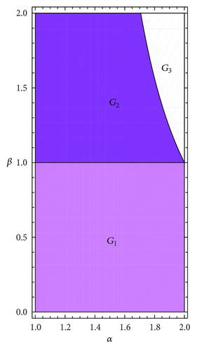
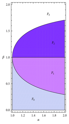
The map Fα,β : [0,1]→[0,1], Fα,β(x) = (fαgβ)(x), in terms of monotonicity, has the following structure in the parametric space (see Figure 1).
  • (i)

    Fα,β is a monotone decreasing map if (α, β) ∈ F0, where

    ()

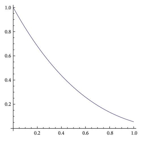
  • see example for α = 1.5 and β = 0.3 in Figure 2(a).

  • (ii)

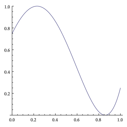
    Fα,β is a unimodal map with a minimum for if (α, β) ∈ F1, where

    ()

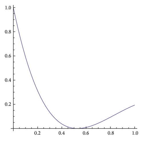
  • see example for α = 1.5 and β = 0.8 in Figure 2(b).

  • (iii)

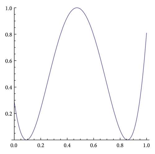
    Fα,β is a bimodal map with a minimum for and a maximum for x = 1/β if (α, β) ∈ F2, where

    ()

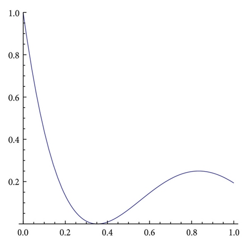
  • see example for α = 1.5 and β = 1.2 in Figure 2(c).

  • (iv)

    Fα,β is a trimodal map with two minima (for and ) and a maximum for x = 1/β if (α, β) ∈ F3, where

    ()

  • see example for α = 1.5 and β = 1.8 in Figure 2(d).
Details are in the caption following the image
Parametric regions for the composition maps Fα,β (a) and Gα,β (b) according to the number of pieces of monotonicity.
Details are in the caption following the image
Parametric regions for the composition maps Fα,β (a) and Gα,β (b) according to the number of pieces of monotonicity.
Details are in the caption following the image
Graphics of the map Fα,β for α = 1.5 and β = 0.3, 0.8, 1.2, and 1.8 for each graphic.
Details are in the caption following the image
Graphics of the map Fα,β for α = 1.5 and β = 0.3, 0.8, 1.2, and 1.8 for each graphic.
Details are in the caption following the image
Graphics of the map Fα,β for α = 1.5 and β = 0.3, 0.8, 1.2, and 1.8 for each graphic.
Details are in the caption following the image
Graphics of the map Fα,β for α = 1.5 and β = 0.3, 0.8, 1.2, and 1.8 for each graphic.
The map Gα,β: [0,1]→[0,1],   Gα,β(x) = (gβfα)(x), has the following structure in the parametric space (see Figure 1).
  • (i)

    Gα,β is a unimodal map with a maximum (for x = 1 − 1/α) if (α, β) ∈ G1, where

    ()

  • see example for α = 1.5 and β = 0.6 in Figure 3(a).

  • (ii)

    Gα,β is a bimodal map with a maximum for x = 1 − 1/α and a minimum for if (α, β) ∈ G2, where

    ()

  • see example for α = 1.3 and β = 1.5 in Figure 3(b).

  • (iii)

    Gα,β is a trimodal map with a maximum for x = 1 − 1/α and two minima in the points and if (α, β) ∈ G3, where

    ()

  • see example for α = 1.9 and β = 1.9 in Figure 3(c).
Details are in the caption following the image
Graphics of the map Gα,β for (a) α = 1.5 and = 0.6, (b) α = 1.3 and β = 1.5, and (c) α = 1.9 and β = 1.9.
Details are in the caption following the image
Graphics of the map Gα,β for (a) α = 1.5 and = 0.6, (b) α = 1.3 and β = 1.5, and (c) α = 1.9 and β = 1.9.
Details are in the caption following the image
Graphics of the map Gα,β for (a) α = 1.5 and = 0.6, (b) α = 1.3 and β = 1.5, and (c) α = 1.9 and β = 1.9.

2.2. Practical Computation of Topological Entropy

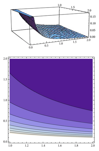
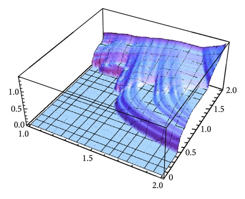
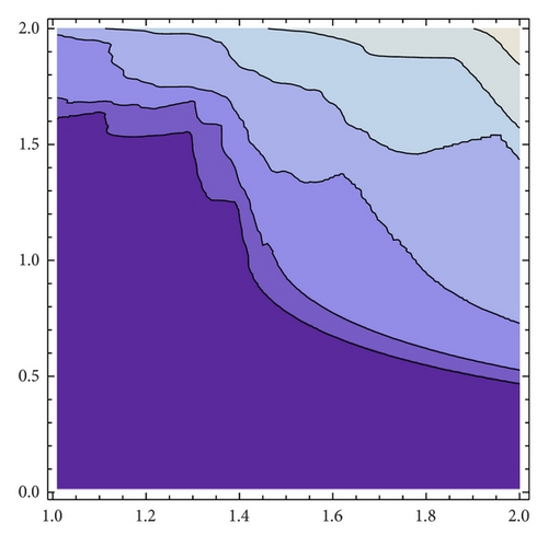
Algorithms for computing the topological entropy for the special case of unimodal maps are given in [6, 7]. An algorithm for bimodal maps (with three pieces of monotonicity) is described in [8], and an algorithm for a particular class of piecewise continuous maps with four pieces of monotonicity is described in [9]. These three types of algorithms cover all the cases involved in the dynamical system that we are considering for the composition maps Fα,β and Gα,β. The results obtained for the model can be observed in Figure 4.
Details are in the caption following the image
Topological entropy with accuracy 10−3 for each (α, β) ∈  [1,2] × [0,2], 3D view (a) and projection (b).
Details are in the caption following the image
Topological entropy with accuracy 10−3 for each (α, β) ∈  [1,2] × [0,2], 3D view (a) and projection (b).

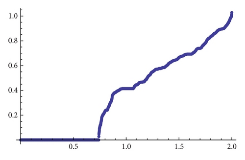
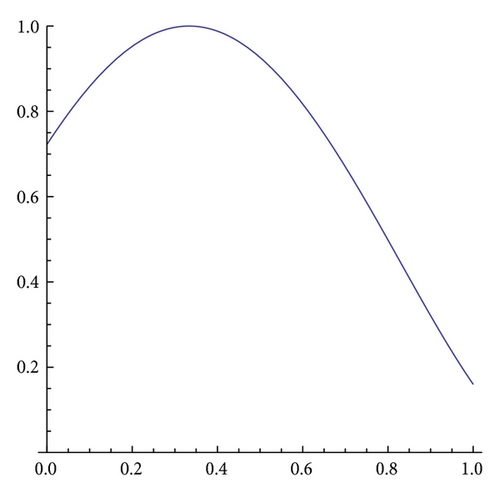
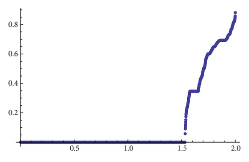
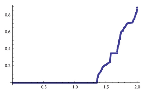
Figures 5(a), 5(b), 5(c), and 5(d) show the topological entropy with accuracy 10−4, where α takes the values 1.25, 1.30, 1.50, and 1.85.
Details are in the caption following the image
Figure 5 (a) Topological entropy for α = 1.25 and accuracy 10−4
Topological entropy for different fixed α  while β ∈ [0,2].
Details are in the caption following the image
Figure 5 (b) Topological entropy for α = 1.30 and accuracy 10−4
Topological entropy for different fixed α  while β ∈ [0,2].
Details are in the caption following the image
Figure 5 (c) Topological entropy for α = 1.50 and accuracy 10−4
Topological entropy for different fixed α  while β ∈ [0,2].
Details are in the caption following the image
Figure 5 (d) Topological entropy for α = 1.85 and accuracy 10−4
Topological entropy for different fixed α  while β ∈ [0,2].

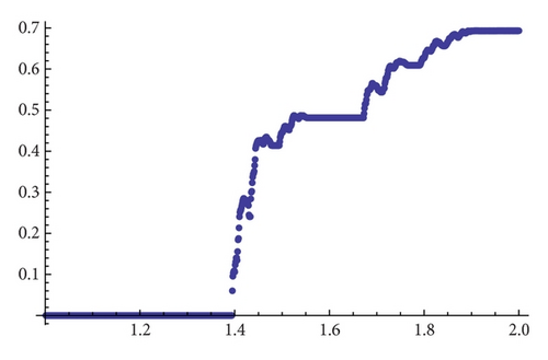
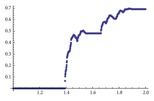
For β = 1.1, and β = 1.15 the topological entropy with accuracy 10−4 is given by Figures 6(a) and 6(b).
Details are in the caption following the image
Figure 6 (a) Topological entropy for β = 1.1 and accuracy 10−4
Topological entropy for fixed β, 1.1 (a) and 1.15 (b) while α ∈ [1,  2].
Details are in the caption following the image
Figure 6 (b) Topological entropy for β = 1.15 and accuracy 10−4
Topological entropy for fixed β, 1.1 (a) and 1.15 (b) while α ∈ [1,  2].

2.3. Existence of Chaotic Maps

Before stating the existence of chaos, we must recall what we understand for chaos. A continuous interval map f : II is chaotic in the sense of Li and Yorke (LY-chaotic) if there is an uncountable set SX (called scrambled set of f) such that for any x, yS, xy, it is held that
()

Positive topological entropy implies chaos in the sense of Blanchard et al. [10], and therefore, the above computations of topological entropy are an analytical proof of the existence of chaos in the model. Even more, we can prove that positive topological entropy is equivalent to chaos in the sense of Li-Yorke. For that, we just need to notice that when the topological entropy is equal to zero, the map is not chaotic because the relative extreme points of the composition maps fαgβ and gβfα are nonflat since the second derivative in these points is nonzero, (remember that a critical point is nonflat if some higher derivative is nonzero). Then, by [11, Theorem A], C maps with nonflat turning points have no wandering intervals (i.e., for a continuous interval map f, an interval J is called wandering if J, f(J), f(J) 2, … are disjoint and no point xJ is asymptotically periodic), and by [12, Lemma 2.7], a map with zero topological entropy is chaotic if and only if it has wandering intervals. Hence, our model is not chaotic when the topological entropy is zero.

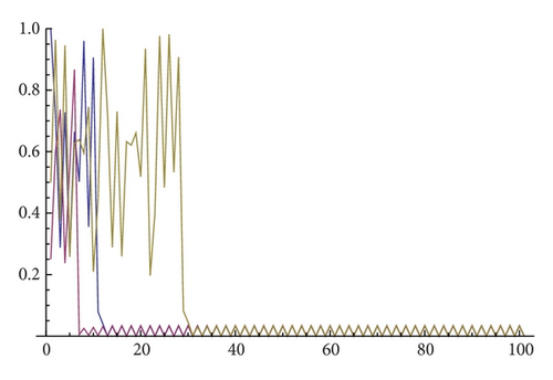
Therefore, we have two regions the nonchaotic one where every trajectory has the property that for any ϵ > 0 there is a periodic trajectory which is ϵ close to it [13]. In practice, one might check that a computer simulation shows the convergence to a periodic orbit when parameters are in the nonchaotic region. For the second region one could expect a similar situation, but as we will show in the next section, the topological chaos we have shown to exist, could not be observed. For instance, for α = 1.8 and β = 1.85, the topological entropy of gβfα is positive, but the time series of several orbits reveal a periodic motion (see Figure 7).
Details are in the caption following the image
We draw a sample of 100 points of three orbits with initial values 0.25, 0.5, and 1 when the parameter values are α = 1.8 and β = 1.85. The picture shows the convergence to a two-periodic orbit which maps 0.033582 to 0.000140067 and vice versa.

3. Chaos, Attractors, and Schwarzian Derivative

We start this section with some useful definitions. Let f : II be a map. A probabilistic measure μ is said to be invariant for f if μ(A) = μ(f−1(A)) for any Borel set AI. In addition, the measure is ergodic if the equality f(A) = A implies that μ(A) = 0 or 1. Denote by (X, f) and (X, f) the set of invariant and ergodic measures of f, respectively.

Given xI, define its ω-limit set ω(x, f) as the set of limits points of its orbit. Recall that a metric attractor is a subset A ⊂ [0,1] such that f(A)⊆A, O(A) = {x : ω(x, f) ⊂ A} has positive Lebesgue measure, and there is no proper subset AA with the same properties. O(A) is called the basin of the attractor.

By [14, Theorem 4.1], for a multimodal map f : II without wandering intervals, there are three possibilities for its metric attractors.
  • (A1)

    A periodic orbit (recall that x is periodic if fn(x) = x for some n).

  • (A2)

    A solenoidal attractor, which is basically a Cantor set in which the dynamics is quasiperiodic. More precisely, the dynamics on the attractor is conjugated to a minimal translation, in which each orbit is dense on the attractor. The dynamics of f restricted to the attractor is simple; neither positive topological entropy nor Li-Yorke chaos can be obtained. Its dynamics is often known as quasiperiodic.

  • (A3)

    A union of periodic intervals, J1, …, Jk, such that fk(Ji) = Ji and fk(Ji) ≠ Jj, 1 ≤ i < jk, and such that fk is topologically mixing. Topologically mixing property implies the existence of dense orbits on each periodic interval (under the iteration of fk).

Moreover, if f has an attractor of types (A2) and (A3), then it must contain the orbit of a turning point, and therefore its number is bounded by the turning points. In the case of our model, we can strengthen the above result by noticing that Fα,β and Gα,β have negative Schwarzian derivative. Namely, the Schwarzian derivative [1517] at a point x is given by
()

Since S(fg)(x) = Sf(g(x))·(g(x)) 2 + Sg(x) and the maps fα and gβ have negative Schwarzian derivative the same occurs to the composition maps Fα,β and Gα,β. Since attractors of type (A1) must also attract the orbit of a turning point when the map has negative Schwarzian derivative, we have that the number of attractors of Fα,β and Gα,β is bounded to at most 3. Even more, when Fα,β and Gα,β have three monotone pieces, then their value in two turning points agree, which implies that in fact, the number of attractors of Fα,β and Gα,β can be at most 2. The following result shows that the attractors of Fα,β and Gα,β are deeply connected.

Proposition 2. Let f, g : II be C1 maps such that ω(x, fg) is an attractor of fg. Then ω(g(x), gf) = g(ω(x, fg)) is an attractor of gf.

Proof. As usual, denote by λ the one-dimensional Lebesgue measure. Let AI with λ(A) > 0 such that for any yA we have ω(y, fg) = ω(x, fg). Since f is C1, we have that λ(f−1(A)) > 0. Now, let zf−1(A), and fix yA such that y = f(z). For any n we have

()
from which we conclude that ω(g(x), gf) = g(ω(x, fg)) is an attractor of gf.

The attractors of the map Rα,β can be obtained by combining the attractors of fαgβ and gβfα. Basically, we must use the inclusion [18, Theorem 2]
()
and, in view of Proposition 2, check whether the attractors of fαgβ and gβfα we are considering are linked or not. In any case, it should be noticed that even when fαgβ and gβfα have just one attractor, the map Rα,β may have several of them depending on their distribution in the XY plane (see, e.g., [18, 19] and the examples of attractors in Figure 12).
Obviously, if fαgβ and gβfα have 2 attractors, the number of different attractors of Rα,β increases. So, still we have a practical work to do to decide whether fαgβ and gβfα have one or two attractors. We fix the map fαgβ and realize that if it has three or four monotone pieces, then the image of its turning points is in {0,1}. We take
()
and converge it to
()
where u and ν are mutually independent ergodic measures of fαgβ (see, e.g., [20]). Since different ergodic measures must be supported in different attractors, when the expression (27) tends to zero when n tends to infinity we have an evidence that just one attractor exists. Hence, we make simulations to compute (27) showing the results in Figure 8. Note that we have to be cautious when 0 or 1 is eventually periodic, because in such case its trajectory ranges all the attractors if the periodic orbit is an attractor, which need not happen (e.g., we can address that the well-known example of the map f(x) = 4x(1 − x) has a dense orbit, and hence, its attractor is the whole interval, and the image of its turning point is 1, which is eventually the fixed point 0). Fortunately, the probability of finding such pathological examples is 0, but this is the case for β = 2 and α > 1.
Details are in the caption following the image
Figure 8 (a) ϵ = 0.1
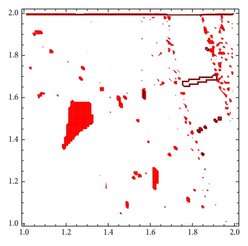
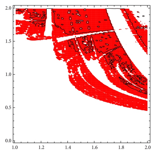
We compute (27) for samples of length n = 10000, 1 < α, β ≤ 2, and constant step size h = 0.01 for both α and β. The parameter α is represented in X-axis. We draw in red the values of (α, β) such that (27) is greater than a fixed value ϵ. In (a) ϵ = 0.1, and for (b) ϵ = 0.01.
Details are in the caption following the image
Figure 8 (b) ϵ = 0.01
We compute (27) for samples of length n = 10000, 1 < α, β ≤ 2, and constant step size h = 0.01 for both α and β. The parameter α is represented in X-axis. We draw in red the values of (α, β) such that (27) is greater than a fixed value ϵ. In (a) ϵ = 0.1, and for (b) ϵ = 0.01.

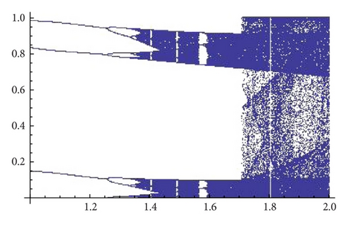
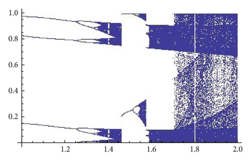
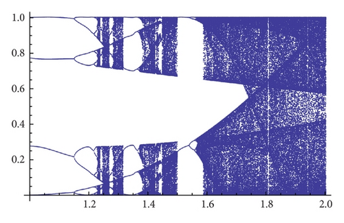
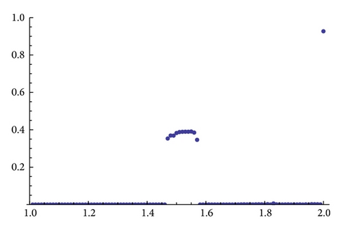
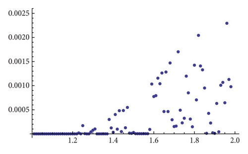
Taking into account the results obtained for generating Figure 8, we see that for α = 1.3 there are values of β around 1.5 for which it seems that two different attractors of Gα,β may coexist. Figure 9 shows a refinement of Figure 8 for α = 1.3 and 1.35. The bifurcation diagrams (see Figure 10) also suggest the existence of two different attractors for α = 1.3 but not for 1.35.
Details are in the caption following the image
(a) We compute (27) for samples of length n = 100000, α = 1.3, 1 < β ≤ 2, and constant step size h = 0.01 for β. We see that (27) is clearly positive when β is in a neighborhood of 1.5. (b) We do the same when α = 1.35, but now we cannot conclude clearly the existence of different attractors.
Details are in the caption following the image
For α = 1.3, (a) and (b) show the bifurcation diagram for initial conditions 0 and 1, respectively. The bifurcation diagrams are constructed with generating orbits of length 100200 and representing just the last 200 points. (c) and (d) show the same when α = 1.35.

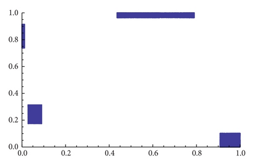
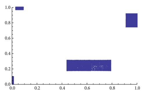
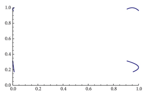
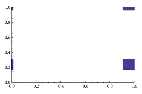
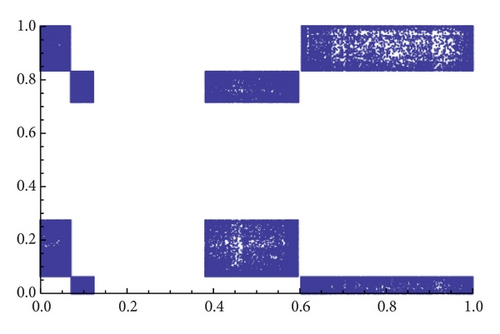
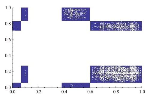
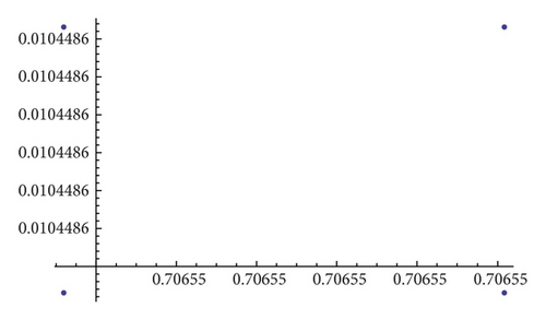
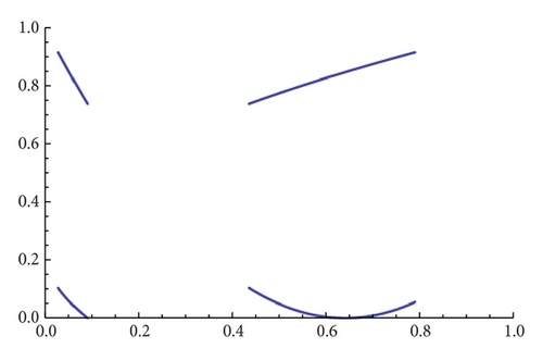
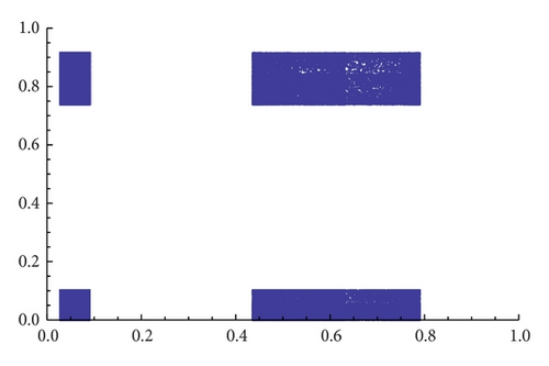
As an example, we show different types of attractors and limit sets (but nonmetric attractors) obtained for the parameter values α = 1.3 and β = 1.56 (see Figure 11 and the explanations therein).
Details are in the caption following the image
Figure 11 (a) x0 = 1/β,   y0 = 0
For α = 1.3 and β = 1.56, we make 200000 iterations and draw the last 100000 in the XY-axis. Except for (b) and (e), the initial conditions are taken to be the extremum of Fα,β and Gα,β. (a) and (e) are not attractors because the initial conditions are synchronized; in (a) gβ(x0) = y0, and in (e) (gβfαgβ(x0)) = y0. These are ω-limit sets from initial conditions in a set of zero two-dimensional Lebesgue measures. If we change the initial conditions slightly, we obtain the attractors (b) and (f). Finally, (c) and (d) are two different attractors with the same projection in the X- and Y-axis, while for (b) and (f) the projections are different. Attractors (b) and (f) are possible because Fα,β and Gα,β have two different attractors consisting of two-periodic transitive intervals (of type (A3)).
Details are in the caption following the image
Figure 11 (b) x0 = 1/β,   y0 = 0.001
For α = 1.3 and β = 1.56, we make 200000 iterations and draw the last 100000 in the XY-axis. Except for (b) and (e), the initial conditions are taken to be the extremum of Fα,β and Gα,β. (a) and (e) are not attractors because the initial conditions are synchronized; in (a) gβ(x0) = y0, and in (e) (gβfαgβ(x0)) = y0. These are ω-limit sets from initial conditions in a set of zero two-dimensional Lebesgue measures. If we change the initial conditions slightly, we obtain the attractors (b) and (f). Finally, (c) and (d) are two different attractors with the same projection in the X- and Y-axis, while for (b) and (f) the projections are different. Attractors (b) and (f) are possible because Fα,β and Gα,β have two different attractors consisting of two-periodic transitive intervals (of type (A3)).
Details are in the caption following the image
Figure 11 (c) x0 = 1/β,   y0 = 1
For α = 1.3 and β = 1.56, we make 200000 iterations and draw the last 100000 in the XY-axis. Except for (b) and (e), the initial conditions are taken to be the extremum of Fα,β and Gα,β. (a) and (e) are not attractors because the initial conditions are synchronized; in (a) gβ(x0) = y0, and in (e) (gβfαgβ(x0)) = y0. These are ω-limit sets from initial conditions in a set of zero two-dimensional Lebesgue measures. If we change the initial conditions slightly, we obtain the attractors (b) and (f). Finally, (c) and (d) are two different attractors with the same projection in the X- and Y-axis, while for (b) and (f) the projections are different. Attractors (b) and (f) are possible because Fα,β and Gα,β have two different attractors consisting of two-periodic transitive intervals (of type (A3)).
Details are in the caption following the image
Figure 11 (d) x0 = 1/β,   y0 = G(1)
For α = 1.3 and β = 1.56, we make 200000 iterations and draw the last 100000 in the XY-axis. Except for (b) and (e), the initial conditions are taken to be the extremum of Fα,β and Gα,β. (a) and (e) are not attractors because the initial conditions are synchronized; in (a) gβ(x0) = y0, and in (e) (gβfαgβ(x0)) = y0. These are ω-limit sets from initial conditions in a set of zero two-dimensional Lebesgue measures. If we change the initial conditions slightly, we obtain the attractors (b) and (f). Finally, (c) and (d) are two different attractors with the same projection in the X- and Y-axis, while for (b) and (f) the projections are different. Attractors (b) and (f) are possible because Fα,β and Gα,β have two different attractors consisting of two-periodic transitive intervals (of type (A3)).
Details are in the caption following the image
Figure 11 (e) x0=1/β(1-1-1/α),  y0=1
For α = 1.3 and β = 1.56, we make 200000 iterations and draw the last 100000 in the XY-axis. Except for (b) and (e), the initial conditions are taken to be the extremum of Fα,β and Gα,β. (a) and (e) are not attractors because the initial conditions are synchronized; in (a) gβ(x0) = y0, and in (e) (gβfαgβ(x0)) = y0. These are ω-limit sets from initial conditions in a set of zero two-dimensional Lebesgue measures. If we change the initial conditions slightly, we obtain the attractors (b) and (f). Finally, (c) and (d) are two different attractors with the same projection in the X- and Y-axis, while for (b) and (f) the projections are different. Attractors (b) and (f) are possible because Fα,β and Gα,β have two different attractors consisting of two-periodic transitive intervals (of type (A3)).
Details are in the caption following the image
Figure 11 (f) x0=1/β(1-1-1/α),  y0=0.999
For α = 1.3 and β = 1.56, we make 200000 iterations and draw the last 100000 in the XY-axis. Except for (b) and (e), the initial conditions are taken to be the extremum of Fα,β and Gα,β. (a) and (e) are not attractors because the initial conditions are synchronized; in (a) gβ(x0) = y0, and in (e) (gβfαgβ(x0)) = y0. These are ω-limit sets from initial conditions in a set of zero two-dimensional Lebesgue measures. If we change the initial conditions slightly, we obtain the attractors (b) and (f). Finally, (c) and (d) are two different attractors with the same projection in the X- and Y-axis, while for (b) and (f) the projections are different. Attractors (b) and (f) are possible because Fα,β and Gα,β have two different attractors consisting of two-periodic transitive intervals (of type (A3)).
Details are in the caption following the image
For α = 1.3 and β = 1.2 we make 200000 iterations and draw the last 100000 in the XY axis. We take initial conditions x0 = 1/β in both cases and y0 = 0.001 for (a) and y0 = (gβfα)(0.001) for (b).
Details are in the caption following the image
For α = 1.3 and β = 1.2 we make 200000 iterations and draw the last 100000 in the XY axis. We take initial conditions x0 = 1/β in both cases and y0 = 0.001 for (a) and y0 = (gβfα)(0.001) for (b).

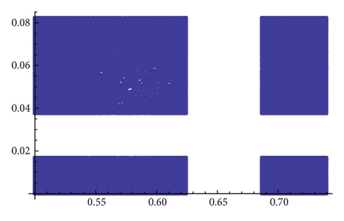
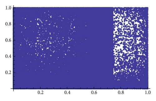
When α = 1.35 the map gβfα seems to have only one attractor, and, for β = 1.2, we see in Figure 12 that several of them may exist (see [18] for an analytical explanation of this fact). Figure 13 shows different types of attractors that can appear when we fix α = 1.86.
Details are in the caption following the image
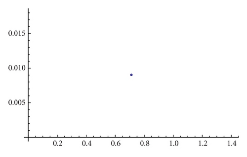
Figure 13 (a) α = 1.86, β = 1.25, x0 = 1/β, and y0 = 1 − 1/α
For α = 1.86 we have drawn several different ω-limits. We make 200000 iterations and draw the last 100000 in the XY axis. We can see that for these parameter values the function is chaotic, but it could happen that the chaos is not physically observable.
Details are in the caption following the image
Figure 13 (b) α = 1.86, β = 1.54, x0 = 1/β, and y0 = 1 − 1/α
For α = 1.86 we have drawn several different ω-limits. We make 200000 iterations and draw the last 100000 in the XY axis. We can see that for these parameter values the function is chaotic, but it could happen that the chaos is not physically observable.
Details are in the caption following the image
Figure 13 (c) α = 1.86, β = 1.56, x0 = 1/β, and y0 = 1 − 1/α
For α = 1.86 we have drawn several different ω-limits. We make 200000 iterations and draw the last 100000 in the XY axis. We can see that for these parameter values the function is chaotic, but it could happen that the chaos is not physically observable.
Details are in the caption following the image
Figure 13 (d) α = 1.86, β = 1.74, x0 = 1/β, and y0 = 1 − 1/α
For α = 1.86 we have drawn several different ω-limits. We make 200000 iterations and draw the last 100000 in the XY axis. We can see that for these parameter values the function is chaotic, but it could happen that the chaos is not physically observable.
Once we have described the attractors of Rα,β, we go back to the idea of explaining when topological chaos cannot be physically observed. To that end, it is worth to notice that for a C1 interval map f, a periodic point xI of period p is an attractor when , and therefore, its Lyapunov exponent (see, e.g., [14]) is
()
Since turning points characterize the attractors of fαgβ and gβfα, we conclude that attractors of type (A3) may exist if and only if λ(gβfα)(c) > 0 for some turning point c of gβfα. The following graphic shows the maximum Lyapunov exponent for the parametric region. Figure 14 shows the maximum of {λ(gβfα)(ci),   i = 1,2}, where c1 and c2 are the turning points that have different forward images by gβfα.
Details are in the caption following the image
We take orbits of length n = 10000 of gβfα with initial conditions on the image of the turning points and estimate the Lyapunov exponent for (α, β) ∈ [1,2] × [0,2] with step size of 0.01. In red we draw those values of the parameter for which the maximum of Lyapunov exponents for the turning points is smaller than or equal to 0.

It is observed that there is a white band in the upper right side of the projection; this corresponds with the region where the fixed point is a local attractor. The topological entropy in these points is positive, but the chaos is not physically observable. Figure 14 explains the results obtained in Figure 7 because the parameter values α = 1.8 and β = 1.85 are clearly in a region with negative Lyapunov exponents.

4. On Invariant Measures and Average Profits

One of the main results in [1] states that for α = 2 and β = 2 the map Rα,β has an invariant measure μ which is absolutely continuous with respect to the two-dimensional Lebesgue measure. Such invariant measure is supported on the whole square [0,1] 2, and therefore, for almost every initial condition, (x, y) (up to a set of zero Lebesgue measure) holds that
()
where Π = (Π1, Π2) is the profit function. Therefore, even when its dynamics is chaotic, with probability one, the average profit can be estimated, and it decided whether the chaotic regime is more profitable than profits at equilibrium points or not. The same estimations can be done also for other economic quantities like production or costs.
The aim of this section is to prove that we can state the same result for a wide range of parameter values of α and β. Note that now we have to take into account several facts.
  • (i)

    The map Rα,β may have several attractors. Therefore, we can have several average values.

  • (ii)

    When we are in the basis of a periodic attractor A = {(x1, y1), …, (xk, yk)}, the equality

    ()

  • trivially holds. Therefore, we must concentrate on attractors constructed from types (A2) and (A3).

  • (iii)

    Since, computationally, attractors of type (A2) are not easily detected and their probability is small, we must concentrate our efforts on deciding when attractors of type (A3) support an invariant ergodic measure which is absolutely continuous with respect to the Lebesgue measure. Note that, by, for example, [21], the existence of dense orbits is not enough to guarantee the existence of absolutely continuous ergodic measures.

We start with the next result, which states that absolutely continuous ergodic measures of fαgβ and gβfα are deeply connected.

Proposition 3. Let f, g : II be C1 maps, and let μ(I, fg) be absolutely continuous with respect to the Lebesgue measure. Then defined by for every Borel set A is an absolutely continuous ergodic measure of gf.

Proof. The fact that can be seen in [22]. Now, let h be a density function for μ; that is, μ(A) = ∫Ah  dλ for any Borel set A. Since

()
we conclude that hf is the density function of , and the proof ends.

Proposition 3 is a great help in detecting the absolutely continuous ergodic measures of Rα,β; we just consider one map Fα,β or Gα,β and decide whether they have absolutely continuous ergodic measures. The absolutely continuous ergodic measures of Rα,β will be constructed by applying Proposition 3 and taking the product measure, which will be absolutely continuous but probably not ergodic. If we denote the product measure by μ1 × μ2, we take the ergodic decomposition , where , and k is the number of different attractors constructed by the attractors of Fα,β and Gα,β supporting the measures μ1 and μ2. The absolutely continuous ergodic measures are therefore ν1, …, νk. In the case studied in [1] we find that k = 1.

So, we fix a turning point of Fα,β for instance and compute its Lyapunov exponent λ(Fα,β)(c). If it is negative or zero, there is nothing to do. So, we assume that it is positive and let J1, …, Jk be periodic intervals such that is an attractor of type (A3). Any ergodic measure μ supported on must satisfy μ(Ji) = 1/k, i = 1, …, k, and then we can consider , the invariant subinterval Ji for some 1 ≤ ik, and the ergodic measure (for ) ν given by the formula ν(A) = μ(AJi) · k. Since has negative Schwarzian derivative, by [23], we conclude that ν, and therefore, μ, can be chosen to be absolutely continuous with respect to the one-dimensional Lebesgue measure.

For instance, we consider the values α = 1.3 and β = 1.56. The possible attractors were studied in detail in Figure 11, and we obtained the following average profits for the initial values as we showed in Table 1.

Table 1. We compute average profits for the initial conditions considered in Figure 11 and following the iteration processes we make there we check that both firms should produce starting from the initial conditions on the basis of the attractor (f). Note that the profits in the fixed point (Cournot equilibrium) are 0.0140236 for firm 1 and 0.148848 for firm 2, and therefore, the only firm interested in stabilizing the Cournot point will be firm 2.
Initial conditions Firm 1 Firm 2
x0 = 1/β, y0 = 0 0.0179073 0.0175666
x0 = 1/β, y0 = 0.001 0.0145578 0.0161027
x0 = 1/β, y0 = 1 −0.00460741 0.052774
x0 = 1/β, y0 = G(1) −0.00459554 0.0527484
0.00177609 0.125768
0.00190711 0.12623

We compute the average profit for each firm. This result could be different if we change initial conditions when the number of attractors is different from one, as we studied in the previous section. Thus, for each firm we are going to present two different graphics in the square (α, β) ∈ [1,2]2 with two different initial conditions, and we observe the differences between them. In the square (α, β)∈[1,2]×[0,1] there is only at most one turning point. Then we study the number of fixed Cournot points depending on (α, β)∈[1,2]×[0,2]. When there are more than a fixed point we determine in which fixed point the profit is maximum for each firm. Finally we compare the average profit with the profit in the fixed point (in which it is maximum) and compute the residual profit.

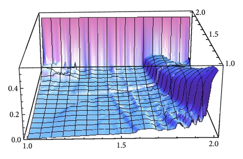
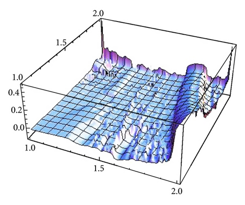
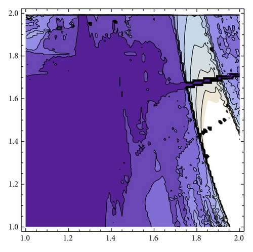
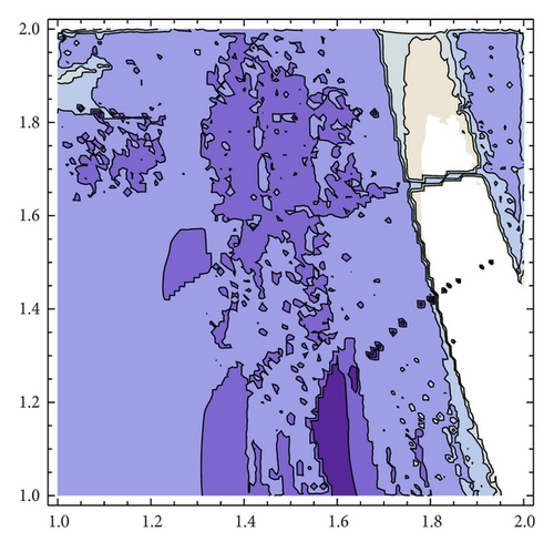
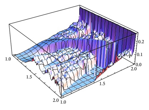
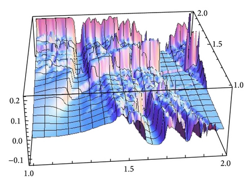
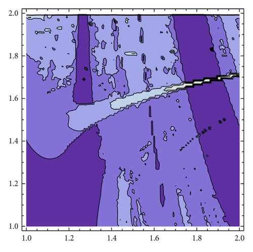
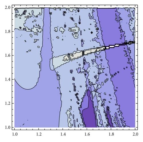
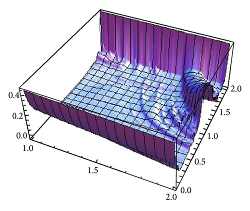
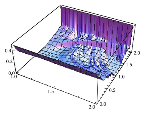
Figure 15 shows the average profit of both firms. For that, we use orbits of length n = 10000 and, as initial conditions, (x, y), where x is the minimum of fαgβ when it exists and 0.4, otherwise, and y is the maximum of gβfα. We will denote this election of initial conditions as min-max conditions. When β is greater than one there are more turning points which eventually may produce other average profits as it is shown in Figure 16. Here, we show the profit of firm 1, taking as initial conditions (x, y), where x is the maximum of fαgβ and y is the maximum of gβfα, which will be denoted as max-max conditions, and compare the situation with the initial conditions min-max previously computed. Figure 17 shows the same scenario for the second firm.
Details are in the caption following the image
Average profits of firm 1 (a) and firm 2 (b) for n = 10000 and step size for parameters α and β eqal to 0.01. The initial conditions are x0 the maximum of fαgβ and y0 the maximum of gβfα (type max-max).
Details are in the caption following the image
Average profits of firm 1 (a) and firm 2 (b) for n = 10000 and step size for parameters α and β eqal to 0.01. The initial conditions are x0 the maximum of fαgβ and y0 the maximum of gβfα (type max-max).
Details are in the caption following the image
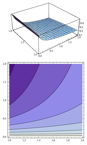
Figure 16 (a) Average profit of firm 1 with min-max initial conditions and β ≥ 1
Average profit for firm 1 with different initial conditions. Note that in projections, the darker the color is, the lower the average profit is.
Details are in the caption following the image
Figure 16 (b) Average profit of firm 1 with max-max initial conditions and β ≥ 1
Average profit for firm 1 with different initial conditions. Note that in projections, the darker the color is, the lower the average profit is.
Details are in the caption following the image
Figure 16 (c) Projection of the average profit of firm 1 with min-max initial conditions
Average profit for firm 1 with different initial conditions. Note that in projections, the darker the color is, the lower the average profit is.
Details are in the caption following the image
Figure 16 (d) Projection of the average profit of firm 1 with max-max initial conditions
Average profit for firm 1 with different initial conditions. Note that in projections, the darker the color is, the lower the average profit is.
Details are in the caption following the image
Figure 17 (a) Average profit of firm 2 with min-max initial conditions and β ≥ 1
Average profit for firm 2 with different initial conditions. Note that in projections, the darker the color is, the lower the average profit is.
Details are in the caption following the image
Figure 17 (b) Average profit of firm 2 with max-max initial conditions and β ≥ 1
Average profit for firm 2 with different initial conditions. Note that in projections, the darker the color is, the lower the average profit is.
Details are in the caption following the image
Figure 17 (c) Projection of the average profit of firm 2 with min-max initial conditions
Average profit for firm 2 with different initial conditions. Note that in projections, the darker the color is, the lower the average profit is.
Details are in the caption following the image
Figure 17 (d) Projection of the average profit of firm 2 with max-max initial conditions
Average profit for firm 2 with different initial conditions. Note that in projections, the darker the color is, the lower the average profit is.

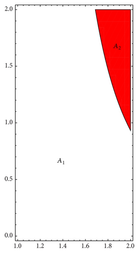
We are interested in analyzing whether the destabilization of Cournot points, even in the chaotic regime, is a good business for both firms. To this end, we compare the average profits of generic orbits with the expected profit at Cournot points. Firstly, we have to compute the number of fixed points of the composition fαgβ, which can be seen in Figure 18. The parameter space can be divided into two regions, A1 and A2. In A1 there is one fixed point while in A2 the number of fixed points is three, which will be ordered x1(α, β) ≤ x2(α, β) ≤ x3(α, β). As an exception, for (α, β) = (2,2), the number of fixed points are four. In [1, Theorems 1 and 2] the stability and bifurcation diagrams of stationary points is studied in detail.
Details are in the caption following the image
Number of fixed points of the composition fαgβ. In A1 there is one fixed point; in A2 there are three fixed points. When (α, β) = (2,2) there are four fixed points.

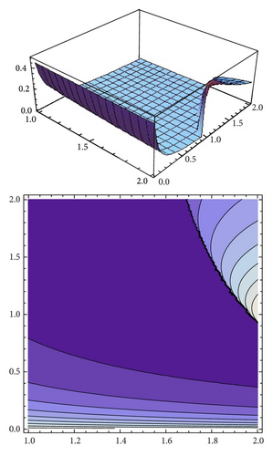
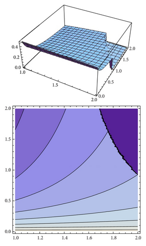
In region A2 we compute the profit of the first firm for each fixed point, and we observe that it is maximum for the fixed point x3(α, β) and minimum for x1(α, β), obtaining the converse situation for the second firm. Figure 19 (resp., Figure 20) shows the profit of the first firm (resp., second firms) against the profit obtained by the second firm (resp., second firm) when the fixed point that maximizes the profit of firm 1 (resp., firm 2) is chosen.
Details are in the caption following the image
Average profits of firms 1 (a) and 2 (b) when we choose the fixed point which gives us the maximum profit of the first firm 1 among all the fixed points. Note that in projections, the darker the color is, the lower the profit is.
Details are in the caption following the image
Average profits of firms 1 (a) and 2 (b) when we choose the fixed point which gives us the maximum profit of the first firm 1 among all the fixed points. Note that in projections, the darker the color is, the lower the profit is.
Details are in the caption following the image
Average profits of firms 1 (a) and 2 (b) when we choose the fixed point which gives us the maximum profit of the first firm 2 among all the fixed points. Note that in projections, the darker the color is, the lower the profit is.
Details are in the caption following the image
Average profits of firms 1 (a) and 2 (b) when we choose the fixed point which gives us the maximum profit of the first firm 2 among all the fixed points. Note that in projections, the darker the color is, the lower the profit is.

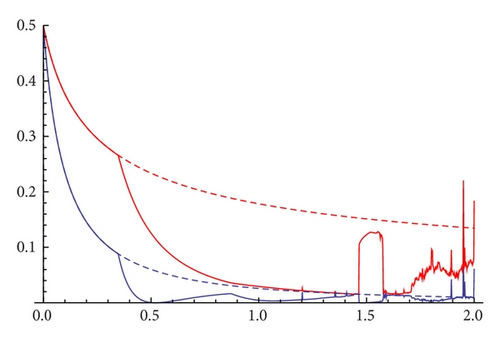
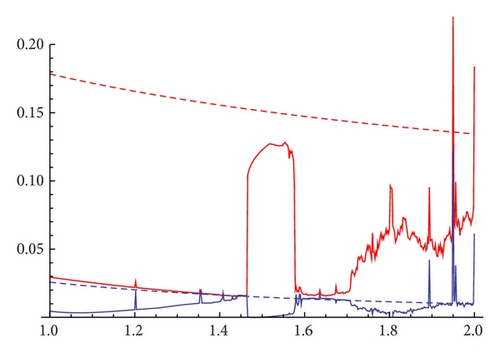
The case α = 1.3 was studied in Figure 11 and Table 1. We compute the profit of both firms in this case to compare the results see Figures 21 and 22.
Details are in the caption following the image
For α = 1.3 and β ∈ (1,2], we show the average profits of firms 1 (blue) and 2 (red) with initial conditions , y0 = 0.999. We also show the profit at the Cournot points for firms 1 (dashed and blue) and 2 (dashed and red). The first figure (a) shows in the X axis the parameter β ∈ [0,2], and the second one (b) with β ∈ [1,2] is a zoom of the first one.
Details are in the caption following the image
In this case α = 1.3, but the initial conditions are x0 = 1/β and y0 = 0.001. The code is the same as in Figure 21. With these initial conditions there are points in which the profit of firm 1 (close to β = 1.56) is greater than the profit reached in the Cournot point.

5. Conclusions

A duopoly model depending on two parameters is studied in detail. By computing its topological entropy we characterize the parameter values which admit the existence of chaotic behavior of trajectories. We also analyze when the above mentioned chaotic trajectories either can be observed or remain on a set of zero Lebesgue measures and therefore are not physically observed in computer simulations. For that, we study the metric attractors of the model concluding that several of them can coexist. The existence of absolutely continuous ergodic measures is proved, and we showed that, even when chaotic maps are considered, the average of economic functions, like profit and production and along the orbits can attain a finite number of values. The existence of such values allows us to make decisions on whether the equilibrium points deserve to be stabilized by choosing strategies that are distinct from naive expectations.

Acknowledgments

This paper has been partially supported by Grants MTM2011-23221 from Ministerio de Ciencia e Innovación (Spain) and 08667/PI/08 from Programa de Generación de Conocimiento Científico de Excelencia de la Fundación Séneca, Agencia de Ciencia y Tecnología de la Comunidad Autónoma de la Región de Murcia (II PCTRM 2007-10), and COST Action IS1104 “The EU in the new economic complex geography: models, tools and policy evaluation.”

      The full text of this article hosted at iucr.org is unavailable due to technical difficulties.