We investigate a Hassell-Varley type predator-prey model with stochastic perturbations. By perturbing the growth rate of prey population and death rate of predator population with white noise terms, we construct a stochastic differential equation model to discuss the effects of the environmental noise on the dynamical behaviors. Applying the comparison theorem of stochastic equations and Itô’s formula, the unique positive global solution to the model for any positive initial value is obtained. We find out some sufficient conditions for stochastically asymptotically boundedness, permanence, persistence in mean and extinction of the solution. Furthermore, a series of numerical simulations to illustrate our mathematical findings are presented. The results indicate that the stochastic perturbations do not cause drastic changes of the dynamics in the deterministic model when the noise intensity is small under some conditions, but while the noise intensity is sufficiently large, the species may die out, which does not happen in the deterministic model.

1. Introduction

It is well known that predator-prey interaction is one of basic interspecies relations for ecosystems, and it is also the basic block of more complicated food chain, food web, and biophysical network structure [1]. Because of the universal existence of predator and prey and their importance in ecology, the dynamical relationship between them has long been and will continue to be one of the dominant themes [2, 3].

The classical predator-prey model has received extensive attentions from mathematicians as well as ecologists [4–7], and it can be expressed by a model of nonlinear ordinary differential equations as follows:

()

where N = N(t) and P = P(t) denote the density of prey and predator population at time t, respectively. Parameters b, c, and d are positive constants. b stands for capturing rate of prey by predator, c is conversion rate of prey into predator, and d is the natural death rate of the predator. The function f(N) represents the density-dependent specific growth rate of prey in absence of predator. The amount of prey biomass consumed by each predator per unit of time is described by the functional response g(N, P).

In this paper, we consider the usual logistic form of the growth function for prey in the absence of predator as

()

where r (>0) is the natural growth rate of prey and K (>0) is the environmental carrying capacity. The functional response g(N, P) is taken as

()

which is called the Hassell-Varley type functional response and α ∈ (0,1) is the Hassell-Varley constant [8] and m (>0) stands for half capturing saturation constant. The predator-prey model with Hassell-Varley type functional response has been studied in the ecological literature [6, 9–11].

For more biological motivation in population dynamics, we take into account the density-dependence of predator population. And the corresponding Hassell-Varley type predator-prey model is described by the following form:

()

where hP stands for the density-dependence of the predator population and h > 0.

On the other hand, most natural phenomena do not follow strictly deterministic laws but rather oscillate randomly about some average. So that the population density never attains a fixed value with the advancement of time but rather exhibits continuous oscillation around some average values [12, 13]. In fact, there are many benefits to be gained by using stochastic models because real life is full of random fluctuations (i.e., the effects of noise), which undeniably arise from either environmental variability or internal species. The basic mechanism and factors of population growth like resources and vital rates—birth, death, immigration, and emigration—change nondeterministically due to continuous fluctuations in the environment (e.g., variation in intensity of sunlight, temperature, water level, etc.) [2, 3, 14]. Recent advances in stochastic differential equations enable a lot of authors to introduce noise into the model of physical phenomena, whether it is a random noise in the system of differential equations or environmental fluctuations in parameters [15–31]. So far as our knowledge is concerned, the work of a modified Hassell-Varley type predator-prey model with stochastic perturbations seems rare. Motivated by these, we attempt to study the stochastic behaviors of the modified Hassell-Varley type predation model in a random fluctuating environment.

The organization of this paper is as follows. In Section 2, we present a stochastic model corresponding to the deterministic model (4) and discuss it in detail. In Section 3, we use numerical simulations to reveal the influence of noise on the dynamical behaviors of the model. A brief discussion is given in Section 4.

2. The Stochastic Model and Analysis

In this section, we investigate the effects of fluctuating environments on the dynamical behaviors of model (4). Assuming that random fluctuations in the environment would display themselves as fluctuations in the growth rate of prey population N and in the death rate of predator population P, then the parameters r and d in model (4) can be replaced by

()

In this way, model (4) will be reduced to the following form:

()

where

and

are known as the intensities of environmental noise and

is a standard white noise; that is, B_i(t) (i = 1,2) is a Brownian motion defined in a complete probability space (Ω, ℱ, P) with a filtration

satisfying the usual conditions (i.e., it is right continuous and increasing while ℱ₀ contains all P-null sets) [14].

2.1. Positive and Global Solution

For model (6), there is a positive local solution.

Lemma 1. There is a unique local solution (N(t), P(t)) for t ∈ [0, τ_e) to model (6) almost surely for initial value , where τ_e is the explosion time.

The proof of this lemma is rather standard and hence is omitted.

Lemma 1 only tells us that there is a unique positive local solution to model (6). Next, we show that this solution is global which is more interesting.

In particular, let us consider the one-dimensional stochastic population model

()

there is an explicit solution

()

From model (6), we have

()

By the comparison theorem of stochastic equations [14], we have

a.s. t ∈ [0, τ_e).

Besides, for the following equation

()

there is a unique solution as

()

In model (6), for α ∈ (0,1), we can get

()

then

a.s. t ∈ [0, τ_e).

Consequently, we obtain

()

On the other hand, the equation

()

has a unique solution as follows:

()

Considering the predator population P(t) in model (6), we have

()

By the comparison theorem, we obtain

a.s. t ∈ [0, τ_e); then

()

From the representation of solutions , , , and , we can see that they are all existence for t ∈ [0, ∞); that is, τ_e = ∞. Therefore, we have the following theorem to show that the positive solution of model (6) is global, which is essential for a population system.

Theorem 2. There is a unique positive solution (N(t), P(t)) of model (6) almost surely for any initial value . Moreover there exist functions , , , and defined as (8), (11), (15), and (17) such that

()

2.2. Stochastic Boundedness

In this subsection, we show that the solution (N(t), P(t)) of model (6) with any positive initial value is uniformly bounded in mean.

Theorem 3. The solution (N(t), P(t)) of model (6) with any positive initial value has the property that

()

Proof. From (7), we obtain

()

combining

, then

()

Set

()

then

()

Integrating the above equation from 0 to t, we obtain

()

and taking expectations leads to

()

then

()

By the comparison theorem, we can get

()

Therefore, we obtain

()

This completes the proof.

2.3. The Long Time Behavior

It is well known that the property of permanence is more desirable since it means the long time survival in a population dynamics. Now, the definition of stochastic permanence will be given below [32, 33].

Definition 4. The solution (N(t), P(t)) of model (6) is said to be stochastically permanent, if, for any ɛ ∈ (0,1), there exists a pair of positive constants δ = δ(ɛ) and χ = χ(ɛ) such that, for any initial value , the solution (N(t), P(t)) to model (6) has the properties that

()

Lemma 5. For any initial value , the solution (N(t), P(t)) satisfies that

()

where C = C(θ) is a positive constant and θ, k are arbitrary positive constants satisfying

()

Proof. Set a function

()

for

; using Itô’s formula, we have

()

Choosing a positive constant θ and by Itô’s formula, we get

()

Let k > 0 be sufficiently small such that it satisfies (31); by Itô’s formula, then

()

Based on the following inequality,

()

Therefore, we obtain

()

There exists a positive constant C₀ such that Le^kt(1 + V) ^θ ≤ C₀e^kt; then

()

So, we can get

()

In addition, we know that (N + P) ^θ ≤ 2^θ(N² + P²) ^θ/2; consequently,

()

The proof is complete.

Based on the results of Theorem 3, Lemma 5, and the Chebyshev inequality [14], we can obtain the following theorem.

Theorem 6. Assume that ; the solution of model (6) is stochastically permanent.

In a view of ecology, the coexistence of species may be a good situation. In the following, we consider the stochastic persistence (i.e., stochastic persistence in mean) of the species.

Theorem 7. Assume that holds, for any initial value N₀ > 0; then the solution N(t) to model (6) has the property

()

Proof. Denoting V(N) = ln N and by Itô’s formula, we obtain

()

Then, we have

()

And we get

()

Dividing t on both sides of the previously mentioned inequality yields

()

Letting t → ∞, we know that

()

Then we obtain

()

On the other hand,

()

dividing t on both sides and letting t → ∞, then

()

From the above results, inequality (41) holds.

Theorem 8. Assume that holds and that (N(t), P(t)) is the solution of model (6) for any initial value ; then

()

which are stable in time average.

Proof. Denoting V(P) = ln P and by Itô’s formula, we have

()

Then,

()

Dividing t on both sides yields

()

we obtain

()

Furthermore,

()

then we can get

()

Dividing t on both sides, we obtain

()

2.4. Extinction

From (17), if

, then lim _t→∞P(t) = 0 a.s. Moreover, from Theorem 7 and (49), we know that if

holds, then

()

which implies that there are a T₀ > 0 and a positive constant n₀ such that N(t) > n₀ a.s. for t ≥ T₀. Besides, for all ɛ > 0, there are T > T₀ and Ω_ɛ such that P(Ω_ɛ) ≥ 1 − ɛ and bP(t)/N(t) ≤ ɛ for t ≥ T. Then we obtain

()

which implies that

()

From Theorem 7 and (47), we have

()

Therefore, by the arbitrary of ɛ, we get

()

Combining the above arguments, we can get the theorem as follows.

Theorem 9. Let (N(t), P(t)) be the solution of model (6) with any initial value . If and , then

()

Furthermore, set u(t) = ln N(t) and v(t) = ln P(t); for the first equation of model (6) we have

()

Taking the comparison theorem of stochastic equations and the theory of diffusion processes [14], then lim _t→∞u(t) = −∞ a.s.; that is,

()

Similarly, we obtain

()

If not, then there is a positive constant H such that

()

Hence, for any given ɛ > 0, there exist t₀ and a set Ω_ɛ such that P(Ω_ɛ) ≥ 1 − ɛ and cN(t)/(N(t) + mP^α(t)) ≤ ɛ for t ≥ t₀. Therefore,

()

By the same reasoning as previously stated, we can get lim _t→∞v(t) = −∞ a.s.; that is,

()

There is a contradiction; hence (66) is true.

Based on the above, we obtain the following theorem which means that if the noise satisfies some conditions, then both species N and P of model (6) will die out.

Theorem 10. Let (N(t), P(t)) be the solution of model (6) with any initial value . If , then

()

3. Numerical Simulations

In this section, we perform some numerical simulations for model (6) with environmental noise to illustrate the previously mentioned analytical findings by referring to the method mentioned in Higham [34]. Next, we consider the discretization equations

()

where ξ_1i and ξ_2i (i = 1,2, …, n) are the Gaussian random variables N(0,1).

When choosing the values of parameters r = 2, K = 0.15, b = 0.8, c = 0.5, d = 0.1, m = 0.1, α = 0.2, and h = 0.1 for model (4), which has three equilibria in the positive quadrant, where E₀ = (0,0) (total extinct) and E₁ = (0.15,0) (extinct of the predator or prey only) are saddle points, E^* = (0.023,0.2025) (coexistence of the prey and predator) is globally asymptotically stable. The trajectory of the prey and predator population of model (4) is shown in Figure 1.

Details are in the caption following the image — **Figure 1**
Open in figure viewer PowerPoint

Phase portrait of model (4). Other parameters are taken as r = 2, K = 0.15, b = 0.8, c = 0.5, d = 0.1, m = 0.1, α = 0.2, and h = 0.1. The horizontal axis is prey population N and the vertical axis is predator population P. E₀ = (0,0) and E₁ = (0.15,0) are two saddle points; E^* = (0.023,0.2025) is stable.

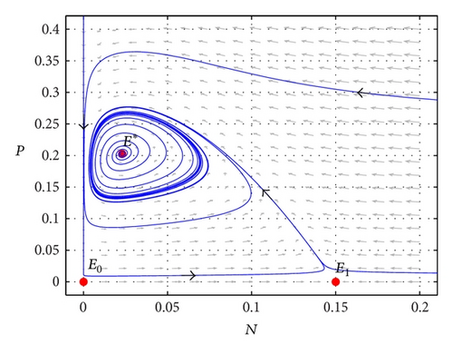
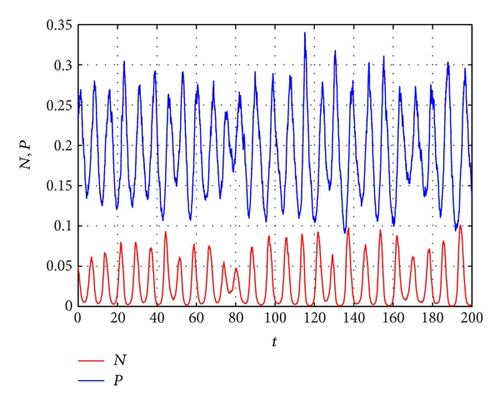
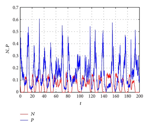
Figure 2 shows the time-series plots of model (6) with different noise intensities and . When choosing σ₁ = σ₂ = 0.045 (Figure 2(a)) and σ₁ = 0.12, σ₂ = 0.3 (Figure 2(b)), from Theorem 6, we know that the positive solution of model (6) is stochastically permanent, which means that stochastic perturbations do not change the permanence of the deterministic model (4). Moreover, from Theorem 7, the model will be stochastically persistent in mean. In other words, we can use the deterministic model (4) describing the dynamics of the stochastic model when the noise intensities and are small. From Figure 2(b), we can observe that the violent fluctuations appear as the noise intensities further increase. It means that noise has strong destabilizing effects on the model and the amplitude of the fluctuations in population density of prey and predator species increases obviously, implying instability of the coexisting equilibrium point in the stochastic environment.

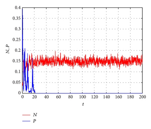
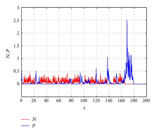
In Figure 3, we continue to choose different noise intensities and to consider the effects of noise to model (6). When choosing σ₁ = 0.15 and σ₂ = 0.9 (Figure 3(a)), the conditions of Theorem 9 are satisfied; then we can find that prey population N(t) of model (6) is permanent and predator population P(t) will die out. Choosing σ₁ = 0.918 and σ₂ = 0.6 in Figure 3(b), which satisfies the conditions of Theorem 10, both species N and P in model (6) become extinct. That is to say, big noise can make the two species die out. From the above numerical results and by Theorems 3, 6, 7, 9, and 10, we conclude that for some noise intensities and the dynamical behaviors of stochastically ultimately boundedness, permanence, persistence in mean, and extinction can be observed in model (6).

4. Conclusions and Remarks

In this paper, we consider a stochastic Hassell-Varley type predator-prey model. The value of this study lies in twofolds. First, it verifies some relevant properties of the corresponding stochastic model (6), which shows the global existence, boundedness and stochastic permanence, persistence in mean, and extinction of the positive solution. Second, it illustrates the dynamics of the model via numerical simulations, which shows that if the noise is not large and satisfies some conditions, the stochastic perturbations do not cause drastic changes of the dynamics in the deterministic model (4), while if the noise is sufficiently large and satisfies some conditions, it will force two species in the model to die out.

In order to study the stochastic model (6), we perturb the deterministic model (4) by incorporating white noise terms in the growth rate of prey population and in the death rate of predator population. Establishing a Lyapunov function, there is a unique positive solution to the model for any positive initial value. Applying Itô’s formula, we derive that, under some conditions, the solution of model (6) is stochastically bounded, permanent, and stochastic persistent in mean and extinct. For the fixed parameters r, K, b, c, d, m, α, and h, some conditions depend on the intensities of noise and noise . When the noise intensities satisfy some conditions of Theorem 9, we can find that prey population N(t) of model (6) is permanent and predator population P(t) will die out (see Figure 3(a)), while with the noise intensities increasing which satisfy the conditions of Theorem 10, from Figure 3(b), two species N and P will die out. In other words, when the noise satisfies some conditions of Theorems 6 and 7 and is not sufficiently large, the populations N and P may be stochastically permanent and persistent in mean, while large noise satisfying the conditions of Theorems 9 and 10 will force the population to become extinct. Our complete analysis of the stochastic model will give some suggestions to the studies of the population dynamics.

Conflict of Interests

The authors declare that there is no conflict of interests regarding the publication of this paper.

Acknowledgments

The authors thank the editor and the anonymous referees for the very helpful suggestions and comments which led to improvement of their original paper. This research was supported by the National Science Foundation of China (no. 11301263).

References

1 Berryman A. A., The origins and evolution of predator-prey theory, Ecology. (1992) 73, no. 5, 1530–1535, 2-s2.0-0027075622.
10.2307/1940005
Web of Science® Google Scholar
2 May R. M., Stability and Complexity in Model Ecosystems, 2001, Princeton University Press, Princeton, NJ, USA.
10.1515/9780691206912
Google Scholar
3 Murray J. D., Mathematical Biology II: Spatial Models and Biomedical Applications, 2003, 18, 3rd edition, Springer, New York, NY, USA, MR1952568.
10.1007/b98869
Google Scholar
4 Beretta E. and Kuang Y., Global analyses in some delayed ratio-dependent predator-prey systems, Nonlinear Analysis. Theory, Methods & Applications. (1998) 32, no. 3, 381–408, https://doi.org/10.1016/S0362-546X(97)00491-4, MR1610586.
10.1016/S0362-546X(97)00491-4
Web of Science® Google Scholar
5 Mischaikow K. and Wolkowicz G., A predator-prey system involving group defense: a connection matrix approach, Nonlinear Analysis. Theory, Methods & Applications. (1990) 14, no. 11, 955–969, https://doi.org/10.1016/0362-546X(90)90112-T, MR1058416.
10.1016/0362-546X(90)90112-T
Web of Science® Google Scholar
6 Cosner C., Deangelis D. L., Ault J. S., and Olson D. B., Effects of spatial grouping on the functional response of predators, Theoretical Population Biology. (1999) 56, no. 1, 65–75, 2-s2.0-0033180314, https://doi.org/10.1006/tpbi.1999.1414.
10.1006/tpbi.1999.1414
CAS PubMed Web of Science® Google Scholar
7 Bandyopadhyay M. and Chattopadhyay J., Ratio-dependent predator-prey model: effect of environmental fluctuation and stability, Nonlinearity. (2005) 18, no. 2, 913–936, https://doi.org/10.1088/0951-7715/18/2/022, MR2122690, ZBL1078.34035.
10.1088/0951-7715/18/2/022
Web of Science® Google Scholar
8 Hassell M. P. and Varley G. C., New inductive population model for insect parasites and its bearing on biological control, Nature. (1969) 223, no. 5211, 1133–1137, 2-s2.0-0014673629, https://doi.org/10.1038/2231133a0.
10.1038/2231133a0
CAS PubMed Web of Science® Google Scholar
9 Abrams P. A. and Ginzburg L. R., The nature of predation: prey dependent, ratio dependent or neither?, Trends in Ecology and Evolution. (2000) 15, no. 8, 337–341, 2-s2.0-0034255819, https://doi.org/10.1016/S0169-5347(00)01908-X.
10.1016/S0169-5347(00)01908-X
CAS PubMed Web of Science® Google Scholar
10 Skalski G. T. and Gilliam J. F., Functional responses with predator interference: viable alternatives to the Holling type II model, Ecology. (2001) 82, no. 11, 3083–3092, 2-s2.0-0035658752.
10.1890/0012-9658(2001)082[3083:FRWPIV]2.0.CO;2
Web of Science® Google Scholar
11 Sutherland W. J., Aggregation and the “ideal free” distribution, The Journal of Animal Ecology. (1983) 52, no. 3, 821–828, 2-s2.0-0021038484.
10.2307/4456
Web of Science® Google Scholar
12 Gard T. C., Persistence in stochastic food web models, Bulletin of Mathematical Biology. (1984) 46, no. 3, 357–370, https://doi.org/10.1016/S0092-8240(84)80044-0, MR748544, ZBL0533.92028.
10.1016/S0092-8240(84)80044-0
Web of Science® Google Scholar
13 Gard T. C., Stability for multispecies population models in random environments, Nonlinear Analysis. Theory, Methods & Applications. (1986) 10, no. 12, 1411–1419, https://doi.org/10.1016/0362-546X(86)90111-2, MR869549, ZBL0598.92017.
10.1016/0362-546X(86)90111-2
Web of Science® Google Scholar
14 Øksendal B. K., Stochastic Differential Equations: An Introduction with Applications, 1995, 4th edition, Springer, New York, NY, USA, MR1411679.
10.1007/978-3-662-03185-8
Google Scholar
15 Liu K. and Mao X., Exponential stability of non-linear stochastic evolution equations, Stochastic Processes and Their Applications. (1998) 78, no. 2, 173–193, https://doi.org/10.1016/S0304-4149(98)00048-9, MR1654577, ZBL0933.60072.
10.1016/S0304-4149(98)00048-9
Web of Science® Google Scholar
16 Sarkar R. R., A stochastic model for autotroph-herbivore system with nutrient reclycing, Ecological Modelling. (2004) 178, no. 3-4, 429–440, 2-s2.0-3242730337, https://doi.org/10.1016/j.ecolmodel.2004.04.013.
10.1016/j.ecolmodel.2004.04.013
Web of Science® Google Scholar
17 Bahar A. and Mao X., Stochastic delay Lotka-Volterra model, Journal of Mathematical Analysis and Applications. (2004) 292, no. 2, 364–380, https://doi.org/10.1016/j.jmaa.2003.12.004, MR2047618, ZBL1043.92034.
10.1016/j.jmaa.2003.12.004
Web of Science® Google Scholar
18 Tornatore E., Buccellato S. M., and Vetro P., Stability of a stochastic SIR system, Physica A. (2005) 354, no. 1–4, 111–126, 2-s2.0-19944381861, https://doi.org/10.1016/j.physa.2005.02.057.
10.1016/j.physa.2005.02.057
Web of Science® Google Scholar
19 Jiang D. Q. and Shi N. Z., A note on nonautonomous logistic equation with random perturbation, Journal of Mathematical Analysis and Applications. (2005) 303, no. 1, 164–172, https://doi.org/10.1016/j.jmaa.2004.08.027, MR2113874, ZBL1076.34062.
10.1016/j.jmaa.2004.08.027
Web of Science® Google Scholar
20 Kooijman S. A. L. M., Grasman J., and Kooi B. W., A new class of non-linear stochastic population models with mass conservation, Mathematical Biosciences. (2007) 210, no. 2, 378–394, https://doi.org/10.1016/j.mbs.2007.05.010, MR2374474.
10.1016/j.mbs.2007.05.010
CAS PubMed Web of Science® Google Scholar
21 Dalal N., Greenhalgh D., and Mao X. R., A stochastic model for internal HIV dynamics, Journal of Mathematical Analysis and Applications. (2008) 341, no. 2, 1084–1101, https://doi.org/10.1016/j.jmaa.2007.11.005, MR2398271, ZBL1132.92015.
10.1016/j.jmaa.2007.11.005
Web of Science® Google Scholar
22 Pang S. L., Deng F. Q., and Mao X. R., Asymptotic properties of stochastic population dynamics, Dynamics of Continuous, Discrete & Impulsive Systems A. (2008) 15, no. 5, 603–620, MR2446028, ZBL1171.34038.
Google Scholar
23 Rao F., Wang W. M., and Li Z. Q., Spatiotemporal complexity of a predator-prey system with the effect of noise and external forcing, Chaos, Solitons & Fractals. (2009) 41, no. 4, 1634–1644, https://doi.org/10.1016/j.chaos.2008.07.005, MR2537770, ZBL1198.34080.
10.1016/j.chaos.2008.07.005
Web of Science® Google Scholar
24 Meng X.-Z., Stability of a novel stochastic epidemic model with double epidemic hypothesis, Applied Mathematics and Computation. (2010) 217, no. 2, 506–515, https://doi.org/10.1016/j.amc.2010.05.083, MR2678562, ZBL1198.92041.
10.1016/j.amc.2010.05.083
Web of Science® Google Scholar
25 Lv J. and Wang K., Asymptotic properties of a stochastic predator-prey system with Holling II functional response, Communications in Nonlinear Science and Numerical Simulation. (2011) 16, no. 10, 4037–4048, https://doi.org/10.1016/j.cnsns.2011.01.015, MR2802710, ZBL1218.92072.
10.1016/j.cnsns.2011.01.015
Web of Science® Google Scholar
26 Ji C. Y., Jiang D. Q., and Li X. Y., Qualitative analysis of a stochastic ratio-dependent predator-prey system, Journal of Computational and Applied Mathematics. (2011) 235, no. 5, 1326–1341, https://doi.org/10.1016/j.cam.2010.08.021, MR2728069, ZBL1229.92076.
10.1016/j.cam.2010.08.021
Web of Science® Google Scholar
27 Wang X. X., Huang H. L., Cai Y. L., and Wang W. M., The complex dynamics of a stochastic predatorprey model, Abstract and Applied Analysis. (2012) 2012, 24, 401031, https://doi.org/10.1155/2012/401031.
10.1155/2012/401031
Google Scholar
28 Liu M. and Wang K., Dynamics of a Leslie-Gower Holling-type II predator-prey system with Lévy jumps, Nonlinear Analysis. Theory, Methods & Applications. (2013) 85, 204–213, https://doi.org/10.1016/j.na.2013.02.018, MR3040360.
10.1016/j.na.2013.02.018
Web of Science® Google Scholar
29 Jiang D., Ji C., Li X., and O′Regan D., Analysis of autonomous Lotka-Volterra competition systems with random perturbation, Journal of Mathematical Analysis and Applications. (2012) 390, no. 2, 582–595, https://doi.org/10.1016/j.jmaa.2011.12.049, MR2890539, ZBL1258.34099.
10.1016/j.jmaa.2011.12.049
Web of Science® Google Scholar
30 Liu M. and Wang K., Analysis of a stochastic autonomous mutualism model, Journal of Mathematical Analysis and Applications. (2013) 402, no. 1, 392–403, https://doi.org/10.1016/j.jmaa.2012.11.043, MR3023266, ZBL06156131.
10.1016/j.jmaa.2012.11.043
Web of Science® Google Scholar
31 Rao F., Dynamical analysis of a stochastic predator-prey model with an Allee effect, Abstract and Applied Analysis. (2013) 2013, 10, 340980, https://doi.org/10.1155/2013/340980.
10.1155/2013/340980
Google Scholar
32 Jiang D. Q., Shi N. Z., and Li X. Y., Global stability and stochastic permanence of a non-autonomous logistic equation with random perturbation, Journal of Mathematical Analysis and Applications. (2008) 340, no. 1, 588–597, https://doi.org/10.1016/j.jmaa.2007.08.014, MR2376180, ZBL1140.60032.
10.1016/j.jmaa.2007.08.014
Web of Science® Google Scholar
33 Li X. Y. and Mao X. R., Population dynamical behavior of non-autonomous Lotka-Volterra competitive system with random perturbation, Discrete and Continuous Dynamical Systems A. (2009) 24, no. 2, 523–545, https://doi.org/10.3934/dcds.2009.24.523, MR2486589, ZBL1161.92048.
10.3934/dcds.2009.24.523
CAS Web of Science® Google Scholar
34 Higham D. J., An algorithmic introduction to numerical simulation of stochastic differential equations, SIAM Review. (2001) 43, no. 3, 525–546, https://doi.org/10.1137/S0036144500378302, MR1872387, ZBL0979.65007.
10.1137/S0036144500378302
Web of Science® Google Scholar

Citing Literature

All articles

Stochastic Analysis of a Hassell-Varley Type Predation Model

Abstract

1. Introduction