
The Itô Integral with respect to an Infinite Dimensional Lévy Process: A Series Approach
Abstract
We present an alternative construction of the infinite dimensional Itô integral with respect to a Hilbert space valued Lévy process. This approach is based on the well-known theory of real-valued stochastic integration, and the respective Itô integral is given by a series of Itô integrals with respect to standard Lévy processes. We also prove that this stochastic integral coincides with the Itô integral that has been developed in the literature.
1. Introduction
The Itô integral with respect to an infinite dimensional Wiener process has been developed in [1–3], and for the more general case of an infinite dimensional square-integrable martingale, it has been defined in [4, 5]. In these references, one first constructs the Itô integral for elementary processes and then extends it via the Itô isometry to a larger space, in which the space of elementary processes is dense.
For stochastic integrals with respect to a Wiener process, series expansions of the Itô integral have been considered, for example, in [6–8]. Moreover, in [9], series expansions have been used in order to define the Itô integral with respect to a Wiener process for deterministic integrands with values in a Banach space. Later, in [10], this theory has been extended to general integrands with values in UMD Banach spaces.
To the best of the author′s knowledge, a series approach for the construction of the Itô integral with respect to an infinite dimensional Lévy process does not exist in the literature so far. The goal of the present paper is to provide such a construction, which is based on the real-valued Itô integral; see, for example, [11–13], and where the Itô integral is given by a series of Itô integrals with respect to real-valued Lévy processes. This approach has the advantage that we can use results from the finite dimensional case, and it might also be beneficial for lecturers teaching students who are already aware of the real-valued Itô integral and have some background in functional analysis. In particular, it avoids the tedious procedure of proving that elementary processes are dense in the space of integrable processes.
In [14], the stochastic integral with respect to an infinite dimensional Lévy process is defined as a limit of Riemannian sums, and a series expansion is provided. A particular feature of [14] is that stochastic integrals are considered as L2-curves. The connection to the usual Itô integral for a finite dimensional Lévy process has been established in [15]; see also Appendix B in [16]. Furthermore, we point out [17, 18], where the theory of stochastic integration with respect to Lévy processes has been extended to Banach spaces.
The idea to use series expansions for the definition of the stochastic integral has also been utilized in the context of cylindrical processes; see [19] for cylindrical Wiener processes and [20] for cylindrical Lévy processes.
- (i)
For an H-valued process X (with H denoting a separable Hilbert space) and a real-valued square-integrable martingale M, we define the Itô integral
(1)where (fk) k∈ℕ denotes an orthonormal basis of H, and 〈X, fk〉 H · M denotes the real-valued Itô integral. We will show that this definition does not depend on the choice of the orthonormal basis. - (ii)
Based on the just defined integral, for an ℓ2(H)-valued process X and a sequence (Mj) j∈ℕ of standard Lévy processes, we define the Itô integral as
(2)For this, we will ensure convergence of the series. - (iii)
In the next step, let L denote an -valued Lévy process, where is a weighted space of sequences (cf. [21]). From the Lévy process L, we can construct a sequence (Mj) j∈ℕ of standard Lévy processes, and for a ℓ2(H)-valued process X, we define the Itô integral
(3) - (iv)
Finally, let L be a general Lévy process on some separable Hilbert space U with covariance operator Q. Then, there exist sequences of eigenvalues (λj) j∈ℕ and eigenvectors, which diagonalize the operator Q. Denoting by an appropriate space of Hilbert Schmidt operators from U to H, our idea is to utilize the integral from the previous step and to define the Itô integral for a -valued process X as
(4)where and are isometric isomorphisms such that Φ(L) is an -valued Lévy process. We will show that this definition does not depend on the choice of the eigenvalues and eigenvectors.
The remainder of this text is organized as follows. In Section 2, we provide the required preliminaries and notation. After that, we start with the construction of the Itô integral as outlined earlier. In Section 3, we define the Itô integral for H-valued processes with respect to a real-valued square-integrable martingale, and in Section 4, we define the Itô integral for ℓ2(H)-valued processes with respect to a sequence of standard Lévy processes. Section 5 gives a brief overview about Lévy processes in Hilbert spaces, together with the required results. Then, in Section 6, we define the Itô integral for ℓ2(H)-valued processes with respect to an -valued Lévy process, and in Section 7, we define the Itô integral in the general case, where the integrand is an -valued process and the integrator a general Lévy process on some separable Hilbert space U. We also prove the mentioned series representation of the stochastic integral and show that it coincides with the usual Itô integral, which has been developed in [5].
2. Preliminaries and Notation
In this section, we provide the required preliminary results and some basic notation. Throughout this text, let (Ω, ℱ, (ℱt) t≥0, ℙ) be a filtered probability space satisfying the usual conditions. For the upcoming results, let E be a separable Banach space, and let T > 0 be a finite time horizon.
Definition 1. Let p ≥ 1 be arbitrary.
- (1)
We define the Lebesgue space
(5)where 𝔻([0, T]; E) denotes the Skorokhod space consisting of all càdlàg functions from [0, T] to E, equipped with the supremum norm. - (2)
We denote by the space of all E-valued adapted processes .
- (3)
We denote by the space of all E-valued martingales .
- (4)
We define the factor spaces
(6)(7)where denotes the subspace consisting of all with M = 0 up to indistinguishability.
Remark 2. Let us emphasize the following.
- (1)
Since the Skorokhod space 𝔻([0, T]; E) equipped with the supremum norm is a Banach space, the Lebesgue space equipped with the standard norm
(8)is a Banach space too. - (2)
By the completeness of the filtration (ℱt) t≥0, adaptedness of an element does not depend on the choice of the representative. This ensures that the factor space of adapted processes is well defined.
- (3)
The definition of E-valued martingales relies on the existence of conditional expectation in Banach spaces, which has been established in [1, Proposition 1.10].
The following auxiliary result shows that these inclusions are closed.
Lemma 3. Let p ≥ 1 be arbitrary. Then, the following statements are true:
- (1)
is closed in ;
- (2)
is closed in .
Proof. Let be a sequence, and let be such that Mn → M in . Furthermore, let τ ≤ T be a bounded stopping time. Then, we have
Now, let be a sequence, and let be such that Xn → X in . Then, for each t ∈ [0, T], we have
Lemma 4. Let H be a separable Hilbert space, and let (hn) n∈ℕ ⊂ H be a sequence with 〈hn, hm〉 H = 0 for n ≠ m. Then, the following statements are equivalent.
- (1)
The series converges in H.
- (2)
The series ∑n∈ℕ hn converges unconditionally in H.
- (3)
One has .
If the previous conditions are satisfied, then one has
3. The Itô Integral with respect to a Real-Valued Square-Integrable Martingale
In this section, we define the Itô integral for Hilbert space valued processes with respect to a real-valued, square-integrable martingale, which is based on the real-valued Itô integral.
In what follows, let H be a separable Hilbert space, and let T > 0 be a finite time horizon. Furthermore, let be a square-integrable martingale. Recall that the quadratic variation 〈M, M〉 is the (up to indistinguishability) unique real-valued, nondecreasing, predictable process with 〈M, M〉 0 = 0 such that M2 − 〈M, M〉 is a martingale.
Proposition 5. Let X be an H-valued, predictable process with
Proof. Let (fk) k∈ℕ be an orthonormal basis of H. For j, k ∈ ℕ with j ≠ k, we have
Now, let (gk) k∈ℕ be another orthonormal basis of H. We define by
Now, Proposition 5 gives rise to the following definition.
Definition 6. For every H-valued, predictable process X satisfying (17), we define the Itô integral as
According to Proposition 5, definition (31) of the Itô integral is independent of the choice of the orthonormal basis (fk) k∈ℕ, and the integral process X · M belongs to .
Remark 7. As the proof of Proposition 5 shows, the components of the Itô integral X · M are pairwise orthogonal elements of the Hilbert space .
Proposition 8. For every H-valued, predictable process X satisfying (17), one has the Itô isometry
Proof. Let (fk) k∈ℕ be an orthonormal basis of H. According to (19), we have
Proposition 9. Let X be a H-valued simple process of the form
Proof. Let (fk) k∈ℕ be an orthonormal basis of H. Then, for each k ∈ ℕ, the process 〈X, fk〉 is a real-valued simple process with representation
Lemma 10. Let X be a H-valued, predictable process satisfying (17). Then, for every orthonormal basis (fk) k∈ℕ of H, one has
Proof. We define the integral process
Remark 11. As a consequence of the Doob-Meyer decomposition theorem, for two square-integrable martingales , there exists (up to indistinguishability) a unique real-valued, predictable process 〈X, Y〉 with finite variation paths and 〈X, Y〉 0 = 0 such that 〈X, Y〉 H − 〈X, Y〉 is a martingale.
Proposition 12. For every H-valued, predictable process X satisfying (17), one has
Proof. Let (fk) k∈ℕ be an orthonormal basis of H. We define the process 𝕁 : = X · M and the sequence (𝕁n) n∈ℕ of partial sums by
Next, we prove that Mn → M in . Indeed, since
Theorem 13. Let be another square-integrable martingale, and let X, Y be two H-valued, predictable processes satisfying (17) and
Proof . Using Proposition 12 and the identities
Proposition 14. Let be another square-integrable martingale such that 〈M, N〉 = 0, and let X, Y be two H-valued, predictable processes satisfying (17) and (53). Then, one has
4. The Itô Integral with respect to a Sequence of Standard Lévy Processes
Definition 15. A sequence (Mj) j∈ℕ of real-valued Lévy processes is called a sequence of standard Lévy processes if it consists of square-integrable martingales with 〈Mj, Mk〉 t = δjk · t for all j, k ∈ ℕ. Here, δjk denotes the Kronecker delta
For the rest of this section, let (Mj) j∈ℕ be a sequence of standard Lévy processes.
Proposition 16. For every ℓ2(H)-valued, predictable process X with
Proof. For j, k ∈ ℕ with j ≠ k, we have 〈Mj, Mk〉 = 0, and, hence, by Proposition 14, we obtain
Therefore, for a ℓ2(H)-valued, predictable process X satisfying (61) we can define the Itô integral as the series (62).
Remark 17. As the proof of Proposition 16 shows, the components of the Itô integral ∑j∈ℕ Xj · Mj are pairwise orthogonal elements of the Hilbert space .
Proposition 18. For each ℓ2(H)-valued, predictable process X satisfying (61), one has the Itô isometry
Proposition 19. Let X be a ℓ2(H)-valued simple process of the form
Proof . For each j ∈ ℕ, the process Xj is a H-valued simple process having the representation
5. Lévy Processes in Hilbert Spaces
In this section, we provide the required results about Lévy processes in Hilbert spaces. Let U be a separable Hilbert space.
Definition 20. A U-valued càdlàg, adapted process L is called a Lévy process if the following conditions are satisfied.
- (1)
We have L0 = 0.
- (2)
Lt − Ls is independent of ℱs for all s ≤ t.
- (3)
We have for all s ≤ t.
Definition 21. A U-valued Lévy process L with and 𝔼[Lt] = 0 for all t ≥ 0 is called a square-integrable Lévy martingale.
Lemma 22. Let L be a U-valued square-integrable Lévy martingale with covariance operator Q, let V be another separable Hilbert space, and let Φ : U → V be an isometric isomorphism. Then, the process Φ(L) is a V-valued square-integrable Lévy martingale with covariance operator QΦ : = ΦQΦ−1.
Proof . The process Φ(L) is a V-valued càdlàg, adapted process with Φ(L0) = Φ(0) = 0. Let s ≤ t be arbitrary. Then, the random variable Φ(Lt) − Φ(Ls) = Φ(Lt − Ls) is independent of ℱs, and we have
Let t, s ∈ ℝ+ and vi ∈ V, i = 1,2 be arbitrary, and set ui : = Φ−1vi ∈ U, i = 1,2. Then, we have
Proposition 23. Let L be a U-valued square-integrable Lévy martingale with covariance operator Q. Then, the sequence (Mj) j∈ℕ given by
Proof. For each j ∈ ℕ, the process Mj is a real-valued square-integrable Lévy martingale. By (73), for all j, k ∈ ℕ, we obtain
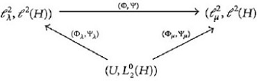
6. The Itô Integral with respect to an -Valued Lévy Process
In this section, we introduce the Itô integral for ℓ2(H)-valued processes with respect to an -valued Lévy process, which is based on the Itô integral (62) from Section 4.
Definition 24. For every ℓ2(H)-valued, predictable process X satisfying (61), we define the Itô integral as
Remark 25. Note that , where denotes the space of Hilbert-Schmidt operators from ℓ2 to H. In [21], the Itô integral for -valued processes with respect to an -valued Wiener process has been constructed in the usual fashion (first for elementary and afterwards for general processes), and then the series representation (88) has been proven; see [21, Proposition 2.2.1].
Now, let (μk) k∈ℕ be another sequence with , and let be an isometric isomorphism such that
is a sequence of standard Lévy processes.
Theorem 26. Let Ψ ∈ L(ℓ2(H)) be an isometric isomorphism such that
Proof. Since Ψ is an isometry, by (61), we have
Remark 27. From a geometric point of view, Theorem 26 says that the “angle” measured by the Itô integral is preserved under isometries.
7. The Itô Integral with respect to a General Lévy Process
In this section, we define the Itô integral with respect to a general Lévy process, which is based on the Itô integral (88) from the previous section.
Lemma 28. The following statements are true.
- (1)
The process Φλ(L) is an -valued square-integrable Lévy martingale with covariance operator .
- (2)
One has
(107)
Proof. By Lemma 22, the process Φλ(L) is an -valued square-integrable Lévy martingale with covariance operator . Furthermore, by (105) and (101), for all j ∈ ℕ, we obtain
Lemma 29. For all h ∈ H and w ∈ ℓ2(H), one has
Proof. By (101) and (111), the vectors and are eigenvectors of Q with corresponding eigenvalues (λj) j∈ℕ and (μk) k∈ℕ. Therefore, for j, k ∈ ℕ with λj ≠ μk, we have . For each , we obtain
Proposition 30. The following statements are true.
Proof. The first two statements follow from Lemma 28. Since Ψλ and Ψμ are isometries, we obtain
By virtue of Proposition 30, Definition (110) of the Itô integral neither depends on the choice of the eigenvalues (λj) j∈ℕ nor on the eigenvectors .
Proposition 32. For every -valued, predictable process X satisfying (109), the process (ξj) j∈ℕ given by
Proof. Since Φλ is an isometry, for each j ∈ ℕ, we obtain
Remark 33. By Remark 17 and the proof of Proposition 32, the components of the Itô integral ∑j∈ℕ ξj · Mj are pairwise orthogonal elements of the Hilbert space .
Proposition 34. For every -valued process X satisfying (109), one has the Itô isometry
Proof. By the Itô isometry (Proposition 18), and since Ψλ is an isometry, we obtain
Proposition 35. Let X be a L(U, H)-valued simple process of the form
Proof. The process is an ℓ2(H)-valued simple process having the representation
Therefore, and since the space of simple processes is dense in the space of all predictable processes satisfying (109); see, for example, [5, Corollary 8.17], the Itô integral (110) coincides with that in [5] for every -valued, predictable process X satisfying (109). In particular, for a driving Wiener process, it coincides with the Itô integral from [1–3].
Acknowledgment
The author is grateful to an anonymous referee for valuable comments and suggestions.