Volume 2013, Issue 1 489295

Research Article

Open Access

A Parameterized Splitting Preconditioner for Generalized Saddle Point Problems

Wei-Hua Luo

School of Mathematical Sciences, University of Electronic Science and Technology of China, Chengdu, Sichuan 611731, China uestc.edu.cn

Key Laboratory of Numerical Simulation of Sichuan Province University, Neijiang Normal University, Neijiang, Sichuan 641112, China njtc.edu.cn

Search for more papers by this author

Ting-Zhu Huang,

Corresponding Author

Ting-Zhu Huang

[email protected]

School of Mathematical Sciences, University of Electronic Science and Technology of China, Chengdu, Sichuan 611731, China uestc.edu.cn

Search for more papers by this author

Wei-Hua Luo,

Wei-Hua Luo

School of Mathematical Sciences, University of Electronic Science and Technology of China, Chengdu, Sichuan 611731, China uestc.edu.cn

Key Laboratory of Numerical Simulation of Sichuan Province University, Neijiang Normal University, Neijiang, Sichuan 641112, China njtc.edu.cn

Search for more papers by this author

Ting-Zhu Huang,

Corresponding Author

Ting-Zhu Huang

[email protected]

School of Mathematical Sciences, University of Electronic Science and Technology of China, Chengdu, Sichuan 611731, China uestc.edu.cn

Search for more papers by this author

First published: 21 April 2013

https://doi.org/10.1155/2013/489295

Academic Editor: P. N. Shivakumar

Share a link

Email
Wechat
Bluesky

Abstract

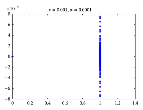
By using Sherman-Morrison-Woodbury formula, we introduce a preconditioner based on parameterized splitting idea for generalized saddle point problems which may be singular and nonsymmetric. By analyzing the eigenvalues of the preconditioned matrix, we find that when α is big enough, it has an eigenvalue at 1 with multiplicity at least n, and the remaining eigenvalues are all located in a unit circle centered at 1. Particularly, when the preconditioner is used in general saddle point problems, it guarantees eigenvalue at 1 with the same multiplicity, and the remaining eigenvalues will tend to 1 as the parameter α → 0. Consequently, this can lead to a good convergence when some GMRES iterative methods are used in Krylov subspace. Numerical results of Stokes problems and Oseen problems are presented to illustrate the behavior of the preconditioner.

1. Introduction

In some scientific and engineering applications, such as finite element methods for solving partial differential equations [1, 2], and computational fluid dynamics [3, 4], we often consider solutions of the generalized saddle point problems of the form

(1)

where A ∈ ℝ^n×n, B ∈ ℝ^m×n (m ≤ n), and C ∈ ℝ^m×m are positive semidefinite, x, f ∈ ℝⁿ, and y, g ∈ ℝ^m. When C = 0, (1) is a general saddle point problem which is also a researching object for many authors.

It is well known that when the matrices A, B, and C are large and sparse, the iterative methods are more efficient and attractive than direct methods assuming that (1) has a good preconditioner. In recent years, a lot of preconditioning techniques have arisen for solving linear system; for example, Saad [5] and Chen [6] have comprehensively surveyed some classical preconditioning techniques, including ILU preconditioner, triangular preconditioner, SPAI preconditioner, multilevel recursive Schur complements preconditioner, and sparse wavelet preconditioner. Particularly, many preconditioning methods for saddle problems have been presented recently, such as dimensional splitting (DS) [7], relaxed dimensional factorization (RDF) [8], splitting preconditioner [9], and Hermitian and skew-Hermitian splitting preconditioner [10].

Among these results, Cao et al. [9] have used splitting idea to give a preconditioner for saddle point problems where the matrix A is symmetric and positive definite and B is of full row rank. According to his preconditioner, the eigenvalues of the preconditioned matrix would tend to 1 when the parameter t → ∞. Consequently, just as we have seen from those examples of [9], preconditioner has guaranteed a good convergence when some iterative methods were used.

In this paper, being motivated by [9], we use the splitting idea to present a preconditioner for the system (1), where A may be nonsymmetric and singular (when rank (B) < m). We find that, when the parameter is big enough, the preconditioned matrix has the eigenvalue at 1 with multiplicity at least n, and the remaining eigenvalues are all located in a unit circle centered at 1. Particularly, when the precondidtioner is used in some general saddle point problems (namely, C = 0), we see that the multiplicity of the eigenvalue at 1 is also at least n, but the remaining eigenvalues will tend to 1 as the parameter α → 0.

The remainder of the paper is organized as follows. In Section 2, we present our preconditioner based on the splitting idea and analyze the bound of eigenvalues of the preconditioned matrix. In Section 3, we use some numerical examples to show the behavior of the new preconditioner. Finally, we draw some conclusions and outline our future work in Section 4.

2. A Parameterized Splitting Preconditioner

Now we consider using splitting idea with a variable parameter to present a preconditioner for the system (1).

Firstly, it is evident that when α ≠ 0, the system (1) is equivalent to

(2)

Let

(3)

Then the coefficient matrix of (2) can be expressed by M − N. Multiplying both sides of system (2) from the left with matrix M⁻¹, we have

(4)

Hence, we obtain a preconditioned linear system from (1) using the idea of splitting and the corresponding preconditioner is

(5)

Now we analyze the eigenvalues of the preconditioned system (4).

Theorem 1. The preconditioned matrix I − M⁻¹N has an eigenvalue at 1 with multiplicity at least n. The remaining eigenvalues λ satisfy

(6)

where s₁ = ω^TBA⁻¹B^Tω, s₂ = ω^TCω, and ω ∈ ℂ^m satisfies

(7)

Proof. Because

(8)

we can easily get

(9)

which implies the preconditioned matrix I − M⁻¹N has an eigenvalue at 1 with multiplicity at least n.

For the remaining eigenvalues, let

(10)

with ∥ω∥ = 1; then we have

(11)

By multiplying both sides of this equality from the left with ω^T, we can get

(12)

This completes the proof of Theorem 1.

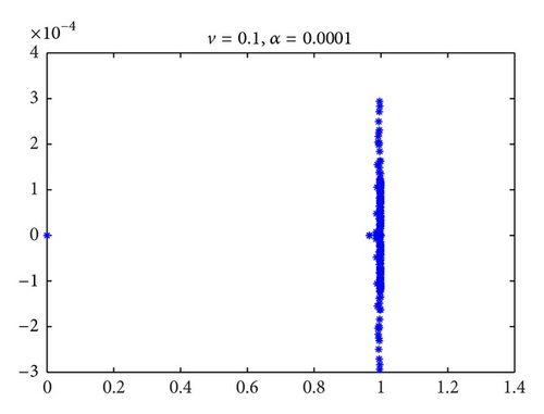
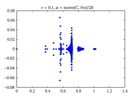
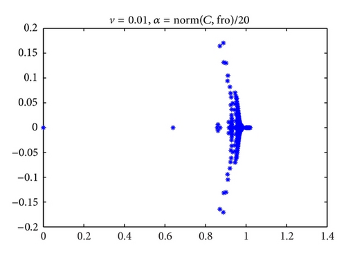
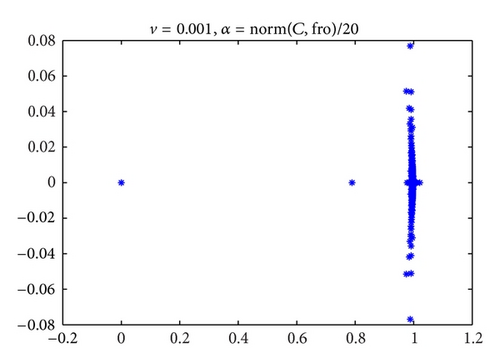
Remark 2. From Theorem 1, we can get that when parameter α is big enough, the modulus of nonnil eigenvalues λ will be located in interval (0,1).

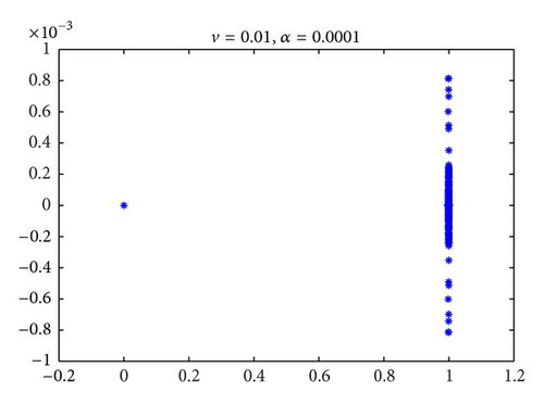
Remark 3. In Theorem 1, if the matrix C = 0, then for nonnil eigenvalues we have

(13)

Figures 1, 2, and 3 are the eigenvalues plots of the preconditioned matrices obtained with our preconditioner. As we can see in the following numerical experiments, this good phenomenon is useful for accelerating convergence of iterative methods in Krylov subspace.

Details are in the caption following the image — **Figure 1 (a)**
Open in figure viewer PowerPoint

Spectrum of the preconditioned steady Oseen matrix with viscosity coefficient v = 0.1, 32 × 32 grid. (a) Q2-Q1 FEM, C = 0; (b) Q1-P0 FEM, C ≠ 0.

Additionally, for the purpose of practically executing our preconditioner

(14)

we should efficiently deal with the computation of (I + (BA⁻¹B^T/α)) ⁻¹. This can been tackled by the well-known Sherman-Morrison-Woodbury formula:

(15)

where A₁ ∈ ℝ^n×n, and

are invertible matrices,

, and

are any matrices, and n, r₁ are any positive integers.

From (15) we immediately get

(16)

In the following numerical examples we will always use (16) to compute (I + (BA⁻¹B^T/α)) ⁻¹ in (14).

3. Numerical Examples

In this section, we give numerical experiments to illustrate the behavior of our preconditioner. The numerical experiments are done by using MATLAB 7.1. The linear systems are obtained by using finite element methods in the Stokes problems and steady Oseen problems, and they are respectively the cases of

(1)
C = 0, which is caused by using Q2-Q1 FEM;
(2)
C ≠ 0, which is caused by using Q1-P0 FEM.

Furthermore, we compare our preconditioner with that of [9] in the case of general saddle point problems (namely, C = 0). For the general saddle point problem, [9] has presented the preconditioner

(17)

with t as a parameter and has proved that when A is symmetric positive definite, the preconditioned matrix has an eigenvalue 1 with multiplicity at n, and the remaining eigenvalues satisfy

(18)

(19)

where σ_i, i = 1,2, …, m, are m positive singular values of the matrix BA^−1/2.

All these systems can be generalized by using IFISS software package [11] (this is a free package that can be downloaded from the site http://www.maths.manchester.ac.uk/~djs/ifiss/). We use restarted GMRES(20) as the Krylov subspace method, and we always take a zero initial guess. The stopping criterion is

(20)

where r_k is the residual vector at the kth iteration.

In the whole course of computation, we always replace in (14) with (16) and use the LU factorization of A + (B^TB/α) to tackle (A + (B^TB/α)) ⁻¹v, where v is a corresponding vector in the iteration. Concretely, let A + (B^TB/α) = LU; then we complete the matrix-vector product (A + (B^TB/α)) ⁻¹v by U∖L∖v in MATLAB term. In the following tables, the denotation norm (C, fro) means the Frobenius form of the matrix C. The total time is the sum of LU time and iterative time, and the LU time is the time to compute LU factorization of A + (B^TB/α).

Case 1 (for our preconditioner). C = 0 (using Q2-Q1 FEM in Stokes problems and steady Oseen problems with different viscosity coefficients. The results are in Tables 1, 2, 3, 4).

Table 1. Preconditioned GMRES(20) on Stokes problems with different grid sizes (uniform grids).

Grid	α	its	LU time	its time	Total time
16 × 16	0.0001	4	0.0457	0.0267	0.0724
32 × 32	0.0001	6	0.3912	0.0813	0.4725
64 × 64	0.0001	9	5.4472	0.5519	5.9991
128 × 128	0.0001	14	91.4698	5.7732	97.2430

Table 2. Preconditioned GMRES(20) on steady Oseen problems with different grid sizes (uniform grids), viscosity v = 0.1.

Grid	α	its	LU time	its time	Total time
16 × 16	0.0001	3	0.0479	0.0244	0.0723
32 × 32	0.0001	3	0.6312	0.0696	0.7009
64 × 64	0.0001	4	13.2959	0.3811	13.6770
128 × 128	0.0001	6	130.5463	3.7727	134.3190

Table 3. Preconditioned GMRES(20) on steady Oseen problems with different grid sizes (uniform grids), viscosity v = 0.01.

Grid	α	its	LU time	its time	Total time
16 × 16	0.0001	2	0.0442	0.0236	0.0678
32 × 32	0.0001	3	0.4160	0.0557	0.4717
64 × 64	0.0001	3	7.3645	0.2623	7.6268
128 × 128	0.0001	4	169.4009	3.1709	172.5718

Table 4. Preconditioned GMRES(20) on steady Oseen problems with different grid sizes (uniform grids), viscosity v = 0.001.

Grid	α	its	LU time	its time	Total time
16 × 16	0.0001	2	0.0481	0.0206	0.0687
32 × 32	0.0001	3	0.4661	0.0585	0.5246
64 × 64	0.0001	3	6.6240	0.2728	6.8969
128 × 128	0.0001	4	177.3130	2.9814	180.2944

Case 1’ (for preconditioner of [9]). C = 0 (using Q2-Q1 FEM in Stokes problems and steady Oseen problems with different viscosity coefficients. The results are in Tables 5, 6, 7, 8).

Table 5. Preconditioned GMRES(20) on Stokes problems with different grid sizes (uniform grids).

Grid	α	its	LU time	its time	Total time
16 × 16	10000	5	0.0471	0.0272	0.0743
32 × 32	10000	7	0.3914	0.0906	0.4820
64 × 64	10000	9	5.6107	0.4145	6.0252
128 × 128	10000	14	92.7154	4.8908	97.6062

Table 6. Preconditioned GMRES(20) on steady Oseen problems with different grid sizes (uniform grids), viscosity v = 0.1.

Grid	α	its	LU time	its time	Total time
16 × 16	10000	4	0.0458	0.0223	0.0681
32 × 32	10000	4	0.5748	0.0670	0.6418
64 × 64	10000	5	12.2642	0.4179	12.6821
128 × 128	10000	7	128.2758	1.6275	129.9033

Table 7. Preconditioned GMRES(20) on steady Oseen problems with different grid sizes (uniform grids), viscosity v = 0.01.

Grid	α	its	LU time	its time	Total time
16 × 16	10000	3	0.0458	0.0224	0.0682
32 × 32	10000	3	0.4309	0.0451	0.4760
64 × 64	10000	4	7.6537	0.1712	7.8249
128 × 128	10000	5	175.1587	3.4554	178.6141

Table 8. Preconditioned GMRES(20) on steady Oseen problems with different grid sizes (uniform grids), viscosity v = 0.001.

Grid	α	its	LU time	its time	Total time
16 × 16	10000	3	0.0507	0.0212	0.0719
32 × 32	10000	3	0.4735	0.0449	0.5184
64 × 64	10000	4	6.6482	0.1645	6.8127
128 × 128	10000	4	172.0516	2.1216	174.1732

Case 2. C ≠ 0 (using Q1-P0 FEM in Stokes problems and steady Oseen problems with different viscosity coefficients. The results are in Tables 9, 10, 11, 12).

Table 9. Preconditioned GMRES(20) on Stokes problems with different grid sizes (uniform grids).

Grid	α	its	LU time	its time	Total time
16 × 16	norm (C, fro)	21	0.0240	0.0473	0.0713
32 × 32	norm (C, fro)	20	0.0890	0.1497	0.2387
64 × 64	norm (C, fro)	20	0.8387	0.6191	1.4578
128 × 128	norm (C, fro)	20	6.8917	3.0866	9.9783

Table 10. Preconditioned GMRES(20) on steady Oseen problems with different grid sizes (uniform grids), viscosity v = 0.1.

Grid	α	its	LU time	its time	Total time
16 × 16	norm (C, fro)/20	10	0.0250	0.0302	0.0552
32 × 32	norm (C, fro)/20	10	0.0816	0.0832	0.1648
64 × 64	norm (C, fro)/20	12	0.8466	0.3648	1.2114
128 × 128	norm (C, fro)/20	14	6.9019	2.0398	8.9417

Table 11. Preconditioned GMRES(20) on steady Oseen problems with different grid sizes (uniform grids), viscosity v = 0.01.

Grid	α	its	LU time	its time	Total time
16 × 16	norm (C, fro)/20	7	0.0238	0.0286	0.0524
32 × 32	norm (C, fro)/20	7	0.0850	0.0552	0.1402
64 × 64	norm (C, fro)/20	11	0.8400	0.3177	1.1577
128 × 128	norm (C, fro)/20	16	6.9537	2.2306	9.1844

Table 12. Preconditioned GMRES(20) on steady Oseen problems with different grid sizes (uniform grids), viscosity v = 0.001.

Grid	α	its	LU time	its time	Total time
16 × 16	norm (C, fro)/20	5	0.0245	0.0250	0.0495
32 × 32	norm (C, fro)/20	5	0.0905	0.0587	0.1492
64 × 64	norm (C, fro)/20	8	1.2916	0.3200	1.6116
128 × 128	norm (C, fro)/20	15	10.4399	2.7468	13.1867

From Tables 1, 2, 3, 4, 5, 6, 7, and 8 we can see that these results are in agreement with the theoretical analyses (13) and (19), respectively. Additionally, comparing with the results in Tables 9, 10, 11, and 12, we find that, although the iterations used in Case 1 (either for the preconditioner of [9] or our preconditioner) are less than those in Case 2, the time spent by Case 1 is much more than that of Case 2. This is because the density of the coefficient matrix generalized by Q2-Q1 FEM is much larger than that generalized by Q1-P0 FEM. This can be partly illustrated by Tables 13 and 14, and the others can be illustrated similarly.

Table 13. Size and number of non-nil elements of the coefficient matrix generalized by using Q2-Q1 FEM in steady Stokes problems.

Grid	dim(A)	nnz(A)	dim(B)	nnz(B)	nnz(A + (1/α)B^TB)
16 × 16	578 × 578	6178	81 × 578	2318	36904
32 × 32	2178 × 2178	28418	289 × 2178	10460	193220
64 × 64	8450 × 8450	122206	1089 × 8450	44314	875966
128 × 128	33282 × 33282	506376	4225 × 33282	184316	3741110

Table 14. Size and number of non-nil elements of the coefficient matrix generalized by using Q1-P0 FEM in steady Stokes problems.

Grid	dim(A)	nnz(A)	dim(B)	nnz(B)	nnz(A + (1/α)B^TB)
16 × 16	578 × 578	3826	256 × 578	1800	7076
32 × 32	2178 × 2178	16818	1024 × 2178	7688	31874
64 × 64	8450 × 8450	70450	4096 × 8450	31752	136582
128 × 128	33282 × 33282	288306	16384 × 33282	129032	567192

4. Conclusions

In this paper, we have introduced a splitting preconditioner for solving generalized saddle point systems. Theoretical analysis showed the modulus of eigenvalues of the preconditioned matrix would be located in interval (0,1) when the parameter is big enough. Particularly when the submatrix C = 0, the eigenvalues will tend to 1 as the parameter α → 0. These performances are tested by some examples, and the results are in agreement with the theoretical analysis.

There are still some future works to be done: how to properly choose a parameter α so that the preconditioned matrix has better properties? How to further precondition submatrix to improve our preconditioner?

Acknowledgments

The authors would express their great thankfulness to the referees and the editor Professor P. N. Shivakumar for their helpful suggestions for revising this paper. The authors would like to thank H. C. Elman, A. Ramage, and D. J. Silvester for their free IFISS software package. This research is supported by Chinese Universities Specialized Research Fund for the Doctoral Program (20110185110020), Sichuan Province Sci. & Tech. Research Project (2012GZX0080), and the Fundamental Research Funds for the Central Universities.

References

1 Brezzi F. and Fortin M., Mixed and Hybrid Finite Element Methods, 1991, 15, Springer, New York, NY, USA, Springer Series in Computational Mathematics, https://doi.org/10.1007/978-1-4612-3172-1, MR1115205, ZBL0788.73002.
10.1007/978-1-4612-3172-1
Google Scholar
2 Chen Z., Du Q., and Zou J., Finite element methods with matching and nonmatching meshes for Maxwell equations with discontinuous coefficients, SIAM Journal on Numerical Analysis. (2000) 37, no. 5, 1542–1570, https://doi.org/10.1137/S0036142998349977, MR1759906, ZBL0964.78017.
10.1137/S0036142998349977
Web of Science® Google Scholar
3 Elman H. C., Silvester D. J., and Wathen A. J., Finite Elements and Fast Iterative Solvers: With Applications in Incompressible Fluid Dynamics, 2005, Oxford University Press, New York, NY, USA, Numerical Mathematics and Scientific Computation, MR2155549.
10.1093/oso/9780198528678.001.0001
Google Scholar
4 Cuvelier C., Segal A., and van Steenhoven A. A., Finite Element Methods and Navier-Stokes Equations, 1986, 22, D. Reidel, Dordrecht, The Netherlands, Mathematics and its Applications, https://doi.org/10.1007/978-94-010-9333-0, MR850259.
10.1007/978-94-010-9333-0
Google Scholar
5 Saad Y., Iterative Methods for Sparse Linear Systems, 2003, 2nd edition, Society for Industrial and Applied Mathematics, Philadelphia, Pa, USA, https://doi.org/10.1137/1.9780898718003, MR1990645.
10.1137/1.9780898718003
Google Scholar
6 Chen K., Matrix Preconditioning Techniques and Applications, 2005, 19, Cambridge University Press, Cambridge, UK, Cambridge Monographs on Applied and Computational Mathematics, https://doi.org/10.1017/CBO9780511543258, MR2169217.
10.1017/CBO9780511543258
Google Scholar
7 Benzi M. and Guo X.-P., A dimensional split preconditioner for Stokes and linearized Navier-Stokes equations, Applied Numerical Mathematics. (2011) 61, no. 1, 66–76, https://doi.org/10.1016/j.apnum.2010.08.005, MR2735256.
10.1016/j.apnum.2010.08.005
Web of Science® Google Scholar
8 Benzi M., Ng M., Niu Q., and Wang Z., A relaxed dimensional factorization preconditioner for the incompressible Navier-Stokes equations, Journal of Computational Physics. (2011) 230, no. 16, 6185–6202, https://doi.org/10.1016/j.jcp.2011.04.001, MR2806221.
10.1016/j.jcp.2011.04.001
Web of Science® Google Scholar
9 Cao Y., Jiang M.-Q., and Zheng Y.-L., A splitting preconditioner for saddle point problems, Numerical Linear Algebra with Applications. (2011) 18, no. 5, 875–895, https://doi.org/10.1002/nla.772, MR2833820, ZBL1249.65065.
10.1002/nla.772
Web of Science® Google Scholar
10 Simoncini V. and Benzi M., Spectral properties of the Hermitian and skew-Hermitian splitting preconditioner for saddle point problems, SIAM Journal on Matrix Analysis and Applications. (2004) 26, no. 2, 377–389, https://doi.org/10.1137/S0895479803434926, MR2124153.
10.1137/S0895479803434926
Web of Science® Google Scholar
11 Elman H. C., Ramage A., and Silvester D. J., Algorithm 886: IFISS, a Matlab toolbox for modelling incompressible flow, ACM Transactions on Mathematical Software. (2007) 33, no. 2, article 14, https://doi.org/10.1145/1236463.1236469, MR2326956.
10.1145/1236463.1236469
Web of Science® Google Scholar

All articles

A Parameterized Splitting Preconditioner for Generalized Saddle Point Problems

Abstract

1. Introduction

2. A Parameterized Splitting Preconditioner

3. Numerical Examples

4. Conclusions

Acknowledgments

References

Figures

References

Information

About Wiley Online Library

Help & Support

Opportunities

Connect with Wiley

A Parameterized Splitting Preconditioner for Generalized Saddle Point Problems

Abstract

1. Introduction

2. A Parameterized Splitting Preconditioner

3. Numerical Examples

4. Conclusions

Acknowledgments

References

Figures

References

Related

Information