The bifurcation properties of a predator prey system with refuge and constant harvesting are investigated. The number of the equilibria and the properties of the system will change due to refuge and harvesting, which leads to the occurrence of several kinds bifurcation phenomena, for example, the saddle-node bifurcation, Bogdanov-Takens bifurcation, Hopf bifurcation, backward bifurcation, separatrix connecting a saddle-node and a saddle bifurcation and heteroclinic bifurcation, and so forth. Our main results reveal much richer dynamics of the system compared to the system with no refuge and harvesting.

1. Introduction

The Holling-Tanner predator-prey system has attracted much attentions from both theoretical and mathematical biologists, especially, in [1] the authors considered the ratio-dependent system of the form

()

where x and y stand for prey and predator population (or densities) at time t, respectively. The predator growth is of logistic type with growth rate r and carrying capacity K in the absence of predation; α and A stand for the predator capturing rate and half saturation constant, respectively; s is the intrinsic growth rate of predator; however, carrying capacity x/b (b is the conversion rate of prey into predators) is the function on the population size of prey. They studied the global properties and the existence and uniqueness of limit cycle for system (1).

Generally speaking, from the views of the optimal management and exploitation of bioeconomic resources, it is necessary and meaningful to consider the refuge or harvesting of populations in some bioeconomic models; one can see [2–11], and the references therein.

In this paper we will analyze the system (1) with refuge and harvesting of the form

()

where r, K, α, A,

, s, and b are positive constants.

is a constant number of prey using refuges, and

is the rate of prey harvesting.

For simplicity, we first rescale the system (2).

Let

, Y = y; system (2) can be written as (still denote X, Y as x, y)

()

Next, let τ = rt, X = x/K, and Y = αy/rK, then system (3) takes the form (still denote X, Y, and τ as x, y, t)

()

where

, a = Ar/α,

, β = α/br, and

From the view of biology, we are only interested in the dynamics of the system (4) in the first quadrant.

The organization of this paper is as follows. In Section 2, we discuss the existence and properties of the equilibria of system (4). In Section 3, all possible bifurcation phenomena of the model in terms of the five parameters are presented, and the numerical simulations about every bifurcation phenomena are exhibited.

2. Qualitative Analysis of Equilibria

To obtain the boundary equilibria the following equation can be obtained

()

Its discriminant is Δ₀ = 1 − 4h.

Obviously, Δ₀ ≥ 0 if 0 < h ≤ 1/4 and Δ₀ < 0 if h > 1/4.

Hence, (5) has two distinct positive solutions , if 0 < m < 1/2, m(1 − m) < h < 1/4, a positive solution x₀₁ if 0 < m < 1,0 < h < m(1 − m), a double solution if 0 < m < 1/2, h = 1/4, and a solution x₀₃ = 1 − 2m when h = m(1 − m) and 0 < m < 1/2.

One can obtain the positive equilibrium of (4) by solving the equation

()

We can derive that system (4) has two positive equilibria P₁ = (x₁, y₁) and P₂ = (x₂, y₂) if

()

where

()

Moreover, we can show that system (4) just exists one positive equilibrium P₁ if 0 < h < m(1 − m) and 0 < m < 1.

The positive equilibrium P₃ = (x₃, y₃) (P_* = (x_*, y_*)) of system (4) exists if 0 < m < (1/2)(1 − β/(aβ + 1)), and h = m(1 − m)(0 < m < (1/2)(1 − β/(aβ + 1)), h = (1/4)(β/(aβ+1)−1)² + mβ/(aβ + 1)), where x₃ = 1 − 2m − β/(aβ + 1), y₃ = βx₃, x_* = −(1/2)(β/(aβ + 1) + 2m − 1), and y_* = βx_*.

Summarizing the previous discussion, the number and location of equilibria of system (4) can be described by the following lemmas.

Lemma 1. Let 1/2 ≤ m < 1.

(i)
System (4) has no equilibria when h ≥ m(1 − m);
(ii)
System (4) exist two equilibria E₁ = (x₀₁, 0) and P₁ when 0 < h < m(1 − m).

Lemma 2. Let 0 < (1/2)(1 − β/(aβ + 1)) ≤ m < 1/2.

(i)
System (4) has no equilibria when h > 1/4.
(ii)
System (4) has a unique equilibrium when h = 1/4.
(iii)
System (4) has two equilibria E₁ = (x₀₁, 0) and E₂ = (x₀₂, 0) when m(1 − m) < h < 1/4.
(iv)
System (4) has an equilibrium E₃ = (x₀₃, 0) when h = m(1 − m).
(v)
System (4) has two equilibria E₁ and P₁ when 0 < h < m(1 − m).

Lemma 3. Let 0 < m < (1/2)(1 − β/(aβ + 1)) and .

(i)
System (4) has no equilibria when h > 1/4.
(ii)
System (4) has a unique equilibrium when h = 1/4.
(iii)
System (4) has two equilibria E₁ and E₂ when .
(iv)
System (4) has three equilibria E₁, E₂, and P_* when .
(v)
System (4) has four equilibria E₁, E₂, P₁, and P₂ when .
(vi)
System (4) has two equilibria E₁ and P₁ when 0 < h < m(1 − m).
(vii)
System (4) has two equilibria E₃ and P₃ when h = m(1 − m).

Next we discuss the dynamics of system (4) in the neighborhood of each feasible equilibria. Firstly, the Jacobian matrix of system (4) at E₁ is

()

It is easy to see that E₁, if exists, is a hyperbolic saddle.

Secondly, the Jacobian matrix of system (4) at E₂ is

()

One can see that boundary equilibrium E₂, if exists, is an unstable hyperbolic node.

The Jacobian matrix of system (4) at E₃ is

()

Hence, E₃, if exists, is a saddle.

Similarly, we assume boundary equilibrium

exists, and the Jacobian matrix of system (4) at

is obtained as follows:

()

Hence, is a saddle node.

The previous discussion can be summarized as follows.

Theorem 4. If the equilibria E₁, E₂, and E₃ exist, then E₁ and E₃ are hyperbolic saddle, and E₂ is a hyperbolic unstable node. Moreover, E₁ and E₂ merge into a saddle node when h = 1/4.

Remark 5. Note that if h = 1/4, then , if h > 1/4, then . Thus, the prey species may go extinct as time increases for some initial values when h ≥ 1/4. That is, biological over harvesting occurs.

In the following, we will discuss the properties of interior equilibria of system (4).

2.1. The Properties of Interior Equilibria

The Jacobian matrix of system (4) at P₁ is

()

The characteristic equation is λ² + A₁λ + A₂ = 0, where

()

Denote that

()

The discriminant of F(δ) = 0 is

, then F(δ) = 0 has two distinct solutions δ₁ and δ₂ denoted by

()

, it is easy to see that P₁ is a node if 0 < δ < δ₁ or δ > δ₂, a degenerate node if δ = δ₁ or δ = δ₂, and a focus or a center type nonhyperbolic if δ₁ < δ < δ₂.

If is a node if δ > δ₂, and a degenerate node if δ = δ₂, and a focus or a center-type nonhyperbolic if 0 < δ < δ₂.

To discuss the stability of P₁, we need to determine the sign of A₁. Define , then .

Clearly, if then A₁ > 0 for all δ; if , then A₁ > 0 when , A₁ ≤ 0 when by simple computation, one can obtain , hence .

The Jacobian matrix of system (4) at P₂ is

()

Its determinant is

Through the previous discussion, about the stability of P₁ and P₂, we have the following theorem.

Theorem 6. Equilibrium P₂, if exists, must be a hyperbolic saddle. Equilibrium P₁, if exists, may be a node or a focus when . And when , P₁ is a stable focus for , a stable degenerate node for δ = δ₂, a stable node for δ > δ₂, an unstable node for 0 < δ < δ₁, an unstable degenerate node for δ = δ₁, an unstable focus for , and a weak focus or a center for .

The Jacobian matrix of system (4) at P₃ is

()

then by the existence condition of P₃,

. Then by taking similar methods used in estimating the properties of P₁, we have the following theorem.

Theorem 7. Let h = m(1 − m), . Then,

(i)
assume 0 < m ≤ (1/2)(1 − β/(1 + aβ) − β/(1+aβ)²), then P₃ is stable;
(ii)
assume (1/2)(1 − β/(1 + aβ) − β/(1+aβ)² ) < m < (1/2)(1 − β/(1 + aβ)), then P₃ is stable if , is unstable if , and is a weak focus or a center if .

The Jacobian matrix of system (4) at P_* is

()

One can see that

, which indicates that P_* is a degenerate singularity and maybe has complicated properties, see the following theorem.

Theorem 8. Let 0 < m < (1/2)(1 − β/(aβ + 1)), . Then system (4) has three equilibria, where E₁ is a hyperbolic saddle, E₂ is a hyperbolic unstable node, and P_* is a degenerate singularity. More precisely,

1^° if δ ≠ 1/(aβ+1)², then P_* is a saddle node;
2^° if δ = 1/(aβ+1)², then P_* is a cusp of codimension 2.

Proof. In order to discuss the properties of system (4) in the neighborhood of the equilibrium P_* = (x_*, y_*), we first take , , then P_* is translated to (0,0), and system (4) becomes (still denote , as x, y)

()

where

()

Clearly, if δ ≠ 1/(aβ+1)² , then

. P_* = (x_*, y_*) is a saddle-node. We finish the proof of the part 1°.

When δ = 1/(aβ+1)² , , which implies that both eigenvalues of the matrix are zero. We rewrite system (20) as

()

where

()

By introducing variable τ = (β/(aβ+1)² )t into previous system and rewriting τ as t for simplicity, then we obtain that

()

where

()

We take transformation X₀ = x, Y₀ = x − (1/β)y into (24), then system (24) is transformed to

()

where

()

In order to obtain the canonical normal forms of system (26), we will perform a series of C^∞ transformations of variables for system (26) in a small neighborhood of (0,0) ^T.

Firstly, performing the transformation by taking X₁ = X₀, , then (26) becomes

()

Secondly, performing the transformation by taking X₂ = X₁, Y₂ = Y₁ + η₅X₁Y₁, then (28) becomes

()

We perform the final transformation of variables by

()

Then, we obtain

()

Note that

()

which indicates that the origin (0,0) of (31) is a cusp of codimension 2. We complete the proof.

3. Bifurcation Analysis

From previous analysis, we can see the equilibria of system (4) may be hyperbolic or degenerate singularities under appropriate conditions, which indicate that some bifurcations may occur for system (4). It is interesting to investigate what kinds of bifurcations system (4) can undergo with the original parameters varying.

3.1. Hopf Bifurcation

Theorem 6 shows that P₁, if exists, is a weak focus or a center when

()

where

To determine the direction of Hopf bifurcation and stability of P₁ in this case, we need to compute the Liapunov coefficients of the equilibrium P₁. Let

and by the variable u = x − x₁, v = y − y₁. Then we rewrite system (4) (still denote u, v as x, y) as follows:

()

We perform the transformations

()

and rewrite u, v as x, y. Then the previous system can be transformed to

()

where the expressions of a₂₀, a₁₁, a₀₂, a₃₀, a₂₁, a₁₂, a₀₃, b₂₀, b₁₁, b₀₂, b₃₀, b₂₁, b₁₂, and b₀₃ depend on the parameters a, β, δ, h, and m, and k₁ =

Using the formula, the first Liapunov number is

()

Therefore, there exists a surface H_b (H_p) in the parameter space (a, m, β, δ, h) which satisfies

()

Hence, when the parameter (a, m, β, δ, h) is in H_b (H_p), the equilibrium P₁ of system (4) is a weak focus of multiplicity 1 and is unstable (stable) (see [8]). H_b (H_p) is called the subcritical (supercritical) Hopf bifurcation surface of system (4).

From Theorem 6, we know that P₁ is a stable focus for and (a, m, β, δ, h) ∈ V, an unstable focus for and (a, m, β, δ, h) ∈ V.

Theorem 9. (i) System (4) has at least one unstable limit cycle if (a, m, β, δ, h) ∈ H_b, , .

(ii) System (4) has at least one stable limit cycle if (a, m, β, δ, h) ∈ H_p, , .

Remark 10. When σ = 0 system (4) maybe undergoes degenerate Hopf bifurcation for some parameter values; since the expression of σ is complicated, we do not discuss this case.

Note that by Theorem 7, if P₃ is a weak focus or a center, then we can obtain that its first Lyapunov number is

()

therefore, P₃ is a stable weak focus.

By numerical calculation, we give the parameter values (a, β, m, h) = (1.6, 2.0, 0.13095, 0.128), then , δ₂ = 0.2220 and k₁σ = 0.31085 > 0, and the existence condition of subcritical Hopf bifurcation is satisfied. If we keep a, β, m, h fixed and choose δ = 0.00249, then a unstable limit cycle can be shown in Figure 1(a).

Details are in the caption following the image — **Figure 1 (a)**
Open in figure viewer PowerPoint

(a) System (4) shows an unstable limit cycle when a = 1.6, β = 2, m = 0.13095, and h = 0.128. ; (b) System (4) shows a stable limit cycle when a = 1.2, β = 2, m = 0.08235, and h = 0.08396. .

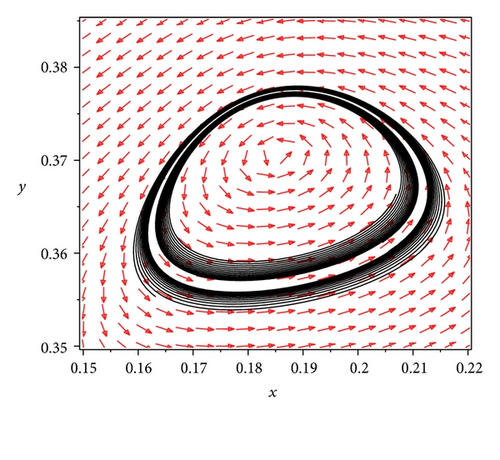
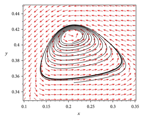
When taking (a, β, m, h) = (1.2, 2.0, 0.08235, 0.08396), then , δ₁ = 0.0000391, and k₁σ = −0.1741543 < 0 which satisfy the existence condition of supercritical Hopf bifurcation. Furthermore, we choose δ = 0.002919; according to Theorem 9, there exists a stable limit cycle, which can be shown in Figure 1(b).

3.2. Backward Bifurcation

Define .

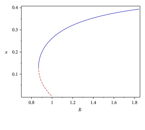
Lemmas 2–3 and Theorems 6–8 illustrate that when the parameter h varies in the range of (0, m(1 − m)], system (4) just has only one positive equilibrium P₁ which is stable. However, when h varies in the range , system (4) has two distinct positive equilibria P₁ and P₂, where P₁ is a stable node or focus and P₂ is a saddle. Furthermore, when , system (4) has unique positive equilibrium P_*. The previous discussion indicates the possibility of a backward bifurcation, which can be summarized as follows.

Theorem 11. Let 0 < m < (1/2)(1 − β/(aβ + 1)), δ > δ₂. Then system (4) has a unique positive equilibrium P_* when R = R_*, has two distinct positive equilibria P₁ and P₂ when R_* < R < 1, where P₁ is a stable node and P₂ is a saddle, and has one positive equilibrium P₁ or P₃ when R ≥ 1. Therefore, system (4) undergoes a backward bifurcation when R = 1.

We give a numerical example in Figure 2 which displays that system (4) has a backward bifurcation at R = 1.

3.3. Saddle-Node Bifurcations

From Lemmas 2–3 and Theorem 4, we see that when 0 < m < 1/2, h = 1/4, E₁ and E₂ degenerate into a saddle-node

. This indicates that there is a saddle node bifurcation surface which takes the form

()

Similarly, from Lemma 3 and the part 1^° of Theorem 8, we know that when 0 < m < (1/2)(1 − β/(aβ + 1)) and , in , system (4) admits the double point P_* = (x_*, y_*). And P_* is a saddle node if δ ≠ 1/(aβ + 1) ².

One also can see that when the parameter h varies in the range of

, system (4) has two distinct positive equilibria P₁ and P₂. From Theorem 6, we know that P₁ may be a stable node, or a focus, and P₂ is a saddle. These imply that system (4) undergoes another saddle-node bifurcation of codimension 1. That is, there is a second saddle-node bifurcation surface SN₂ which is defined by

()

3.4. Bogdanov-Takens Bifurcation

From the part 2^° of Theorem 8, we can see that system (4) exists a cusp of codimension 2, which implies that there may exist the Bogdanov-Takens bifurcation in system (4). Clearly, there exists a parameter space

()

such that system (4) has a cusp of codimension 2 when (m, a, β, h, δ) ∈ BT.

To show that system (4) undergoes the Bogdanov-Takens bifurcation we choose δ and β as bifurcation, parameters. We need to find the universal unfolding of P_*.

Let (m, a, β, h, δ) ∈ BT, and consider the following unfold system

()

where μ₁ and μ₂ are small parameters and vary in the neighborhood of the origin.

Translating P_* to (0,0) by the transformation X = x − x_* and Y = y − y_*. Then system (43) is rewritten as

()

where W₁ and W₂ are smooth functions of X, Y at least of the third order. And

()

Taking the change of variables

and rewriting

as X, Y, we obtain

()

where

()

with μ₁ → 0, μ₂ → 0.

Taking u = X + n₃/n₅, substituting u in system (46), and rewriting u as X, we get that

()

where W₄ is a smooth function of X, Y, and μ at least of order three. When μ₁ → 0, μ₂ → 0,

()

Next, let s = t/(1 − n₆X), x = X, and y = (1 − n₆X)Y into (48) and rewriting s, x, and y as t, X, and Y yields

()

where W₅ is a smooth function of X, Y, and μ at least of order three and

()

when μ₁ → 0, μ₂ → 0. Let

, ν = (ε₃/n₅)t, and rewrite ν as t. Then system (50) becomes

()

where W₆ is a smooth function of x, y, and μ at least of order three and

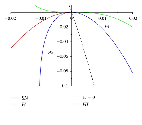
Then system (4) exists the following bifurcation curves in a small neighborhood of the origin in the (μ₁, μ₂) plane.

Theorem 12. Let 0 < m < 1/2 − β/2(aβ + 1), δ = 1/(aβ+1)², h = (1/4)(β/(aβ+1)−1)² + mβ/(aβ + 1). Then system (43) admits the following bifurcations:

(i)
there exists a saddle node bifurcation curve ;
(ii)
there is a Hopf bifurcation curve H = {(μ₁, μ₂) : ε₁ = 0 + o(∥μ∥) ², ε₂ < 0};
(iii)
there is a homoclinic bifurcation curve .

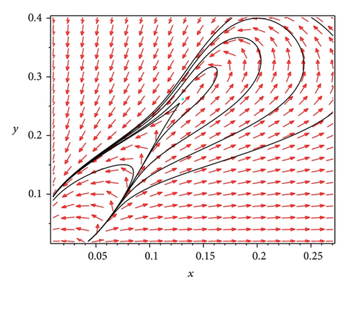
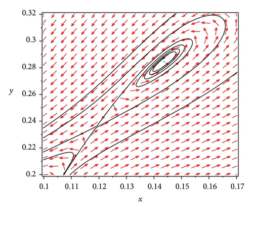
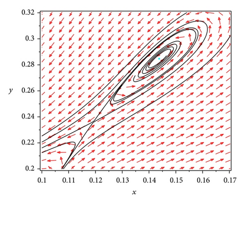
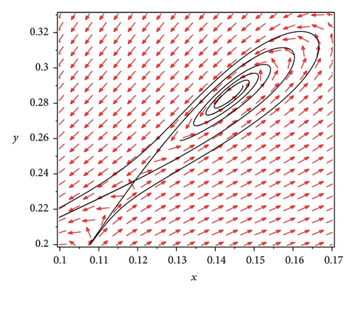
The biological interpretation for the Bogdanov-Takens bifurcation is that if the harvesting rate h and the prey refuge value m satisfy 0 < m < 1/2 − β/2(aβ + 1) , h = (1/4)(β/(aβ+1)−1)² + mβ/(aβ + 1), and δ = 1/(aβ+1)², then the predator and prey coexist in the form of a positive equilibrium or a periodic orbit for different initial values, respectively. And there exist other values of parameters, such that the predator and prey coexist in the form of a positive equilibrium for all initial values lying inside the homoclinic loop, and the predator and prey coexist in the form of a periodic orbit with infinite period for all initial values on the homoclinic loop. By choosing β = 2, a = 1.6, m = (1/4)(1 − β/(aβ + 1)), h = (1/4)(β/(aβ+1)−1)² + mβ/(aβ + 1), and δ = 1/(aβ+1)², the numerical simulations for the Bogdanov-Takens bifurcation in Theorem 12 can be shown in Figures 3, 4 and 5.

3.5. Separatrix Connecting a Saddle-Node and a Saddle Bifurcation and Heteroclinic Bifurcation

From Theorem 8 and Lemma 3, when 0 < m < (1/2)(1 − β/(aβ + 1)), , δ ≠ 1/(aβ + 1) ², there may exist a separatrix connecting the saddle-node P_* and the saddle E₁. When 0 < m < (1/2)(1 − β/(aβ + 1)), , the saddle node P_* separates into the hyperbolic node P₁ and the hyperbolic saddle P₂, which implies that system (4) undergoes a separatrix connecting a saddle node and a saddle bifurcation. Furthermore, the heteroclinic bifurcation may occur if there exists a heteroclinic orbit connecting the separatrix of saddle E₁ and saddle P₂.

Acknowledgments

This paper is supported by NSFC (11226142), Foundation of Henan Educational Committee (2012A110012), Foundation of Henan Normal University (2011QK04, 2012PL03), Natural Science Foundation of Shanghai (12ZR1421600), and Shanghai Municipal Educational Committee (10YZ74).

References

1 Liang Z. and Pan H., Qualitative analysis of a ratio-dependent Holling-Tanner model, Journal of Mathematical Analysis and Applications. (2007) 334, no. 2, 954–964, https://doi.org/10.1016/j.jmaa.2006.12.079, MR2338640, ZBL1124.34030.
10.1016/j.jmaa.2006.12.079
Web of Science® Google Scholar
2 Rebaza J., Dynamics of prey threshold harvesting and refuge, Journal of Computational and Applied Mathematics. (2012) 236, no. 7, 1743–1752, https://doi.org/10.1016/j.cam.2011.10.005, MR2863510, ZBL1235.92048.
10.1016/j.cam.2011.10.005
Web of Science® Google Scholar
3 Gupta R.P. and Chandra P., Bifurcation analysis of modified Leslie-Gower predator–prey model with Michaelis-Menten type prey harvesting, Journal of Mathematical Analysis and Applications. (2013) 398, no. 1, 278–295, https://doi.org/10.1016/j.jmaa.2012.08.057, MR2984333.
10.1016/j.jmaa.2012.08.057
Web of Science® Google Scholar
4 Liu X. and Han M., Chaos and Hopf bifurcation analysis for a two species predator-prey system with prey refuge and diffusion, Nonlinear Analysis. (2011) 12, no. 2, 1047–1061, https://doi.org/10.1016/j.nonrwa.2010.08.027, MR2736192, ZBL1222.34099.
10.1016/j.nonrwa.2010.08.027
Google Scholar
5 Ma Z., Li W., Zhao Y., Wang W., Zhang H., and Li Z., Effects of prey refuges on a predator-prey model with a class of functional responses: the role of refuges, Mathematical Biosciences. (2009) 218, no. 2, 73–79, https://doi.org/10.1016/j.mbs.2008.12.008, MR2513672, ZBL1160.92043.
10.1016/j.mbs.2008.12.008
PubMed Web of Science® Google Scholar
6 Chen L., Chen F., and Chen L., Qualitative analysis of a predator-prey model with Holling type II functional response incorporating a constant prey refuge, Nonlinear Analysis. (2010) 11, no. 1, 246–252, https://doi.org/10.1016/j.nonrwa.2008.10.056, MR2570544, ZBL1186.34062.
10.1016/j.nonrwa.2008.10.056
Google Scholar
7 Xiao D. and Jennings L. S., Bifurcations of a ratio-dependent predator-prey system with constant rate harvesting, SIAM Journal on Applied Mathematics. (2005) 65, no. 3, 737–753, https://doi.org/10.1137/S0036139903428719, MR2136029, ZBL1094.34024.
10.1137/S0036139903428719
Web of Science® Google Scholar
8 Xiao D., Li W., and Han M., Dynamics in a ratio-dependent predator-prey model with predator harvesting, Journal of Mathematical Analysis and Applications. (2006) 324, no. 1, 14–29, https://doi.org/10.1016/j.jmaa.2005.11.048, MR2262452, ZBL1122.34035.
10.1016/j.jmaa.2005.11.048
Web of Science® Google Scholar
9 Wang L.-L., Fan Y.-H., and Li W.-T., Multiple bifurcations in a predator-prey system with monotonic functional response, Applied Mathematics and Computation. (2006) 172, no. 2, 1103–1120, https://doi.org/10.1016/j.amc.2005.03.010, MR2201505, ZBL1102.34031.
10.1016/j.amc.2005.03.010
Web of Science® Google Scholar
10 Tao Y., Wang X., and Song X., Effect of prey refuge on a harvested predator-prey model with generalized functional response, Communications in Nonlinear Science and Numerical Simulation. (2011) 16, no. 2, 1052–1059, https://doi.org/10.1016/j.cnsns.2010.05.026, MR2725826, ZBL1221.34149.
10.1016/j.cnsns.2010.05.026
Web of Science® Google Scholar
11 Berezovskaya F. S., Song B., and Castillo-Chavez C., Role of prey dispersal and refuges on predator-prey dynamics, SIAM Journal on Applied Mathematics. (2010) 70, no. 6, 1821–1839, https://doi.org/10.1137/080730603, MR2596503, ZBL1242.92056.
10.1137/080730603
Web of Science® Google Scholar

Citing Literature

All articles

Bifurcations of a Ratio-Dependent Holling-Tanner System with Refuge and Constant Harvesting

Abstract

1. Introduction

2. Qualitative Analysis of Equilibria

2.1. The Properties of Interior Equilibria