This paper analyses the dynamics of a duopoly with quantity-setting firms and different attitudes towards strategic uncertainty. By following the recent literature on decision making under uncertainty, where the Choquet expected utility theory is adopted to allow firms to plan their strategies, we investigate the effects of the interaction between pessimistic and optimistic firms on economic dynamics described by a two-dimensional map. In particular, the study of the local and global behaviour of the map is performed under three assumptions: (1) both firms have complete information on the market demand and adjust production over time depending on past behaviours (static expectations—“best reply” dynamics); (2) both firms have incomplete information and production is adjusted over time by following a mechanism based on marginal profits; and (3) one firm has incomplete information on the market demand and production decisions are based on the behaviour of marginal profits, and the rival has complete information on the market demand and static expectations. In cases 2 and 3 it is shown that complex dynamics and coexistence of attractors may arise. The analysis is carried forward through numerical simulations and the critical lines technique.

1. Introduction

In this paper, we analyse the dynamics of a Cournot duopoly under strategic uncertainty with pessimistic and optimistic firms within the framework of a nonlinear dynamic oligopoly as those developed by a recent burgeoning literature (see [1] and the papers cited therein).

The issue of decision making under uncertainty as distinct from risk has recently been revisited, amongst others, by [2–6]. In these papers, strategic uncertainty is represented by means of the Choquet expected utility (CEU) theory [7] where agents exhibit different attitudes towards uncertainty, that is, pessimism or optimism, overweighing less or more uncertain events. This theory has also been adopted by [8] to represent strategic behaviour à la Cournot with different firms’ attitude towards uncertainty (CEU theory has been applied to other economic contexts, where optimism and pessimism can explain the paradox of people buying insurance and gambling, the equity premium puzzle, and the small stock puzzle [6]).

In a strategic context such as a duopoly game, it is crucial to forecast the behaviour of the competitor in order to make a decision and to specify the information set available to each player. In the literature on nonlinear oligopolies, two distinct assumptions with regard to available information are usually made: players have a complete knowledge of the market demand and use some form of expectations about the rival’s strategic variable decision (e.g., naive, rational, or adaptive expectations or, alternatively, some weighted sum of previous rules) to set the price or the quantity in the future period (e.g., [9, 10]); players have limited information about the market demand and use some forms of estimation of their own current marginal profits (e.g., [11–14]) or other adjustment mechanisms such as the local monopolistic approximation to determine the price or quantity in the future period [15]. This is because, under the hypothesis of limited information, players are unable to solve the optimisation problem by accounting for expectations about the value of the strategic variable that the competitor will choose for the next period, but they are able to get either a correct estimate of the slope of their own profit function in the current period, that is, the partial derivative of the profit function computed at the current state of production, or use a linear approximation of the demand function by market experiments without any guess about the influence of the competitors (i.e., monopolistic approximation).

In this paper we study local and global dynamics of a Cournot duopoly model with strategic uncertainty as in [8] by considering different information sets of players. In particular, (1) both firms have complete information on the market demand and use the “best reply” adjustment mechanism (static expectations) to vary production period by period; (2) both firms have incomplete information on the market demand and adjust production by following a mechanism based on marginal profits; (3) one firm has incomplete information and production decisions are based on the behaviour of marginal profits, and the rival has complete information and static expectations. These assumptions make the topological structure of the map different and then comparing the local and global properties of the three dynamic systems is relevant. In particular, in cases 2 and 3 we find that complex dynamics as well as coexistence of attractors may occur. These phenomena depend on the relative value of the parameter that weights the strategic uncertainty of firms. The analysis is performed by applying the critical lines techniques as well as through numerical simulations.

The rest of the paper proceeds as follows. Section 2 develops the Cournot model with strategic uncertainty. Section 3 studies the dynamics of the model under complete information and static expectations of both firms. Section 4 introduces the adjustment mechanism of production based on marginal profits for both firms and performs the local and global dynamics. Section 5 analyses the mixed case. Section 6 outlines the conclusions.

2. The Model

We consider a Cournot duopoly for a single homogenous product with a liner negatively sloped inverse demand given by

(1)

where a, b > 0, p > 0 denotes the consumers’ marginal willingness to pay for product Q = q₁ + q₂, and q₁ (resp., q₂) is the output produced by firm 1 (resp., firm 2). The average and marginal costs for each single firm to provide one additional unit of output in the market are equal and given by 0 < c < a.

Profits of firm i = {1,2}, Π_i, can be written as follows:

(2)

We assume that firms are risk neutral and their single productive capacity is able to satisfy the whole market. With regard to strategic uncertainty, each firm does not know whether the rival behaves as a quantity setter à la Cournot. However, each firm has some beliefs about rival’s behaviour and such beliefs are different because each firm has a specific attitude, that is, it is either pessimistic or optimistic, towards uncertainty. In particular, we assume that the pessimistic firm assigns a positive probability of being in the worst case (which is realised when the market price equals zero) (the firm considers it possible that the supply of the other firm is large enough to get the price to zero), while the optimistic firm assigns a positive probability of being in the best case, (which is realised when it behaves as a monopolist in the market).

By using CEU theory, it is assumed that each firm maximises its own CEU function which is given by a weighted average (with the parameter γ ∈ [0,1]) of its expected profits and the profits in the worst case (resp., best case) for the pessimistic (resp., optimistic) firm, where γ (assumed to be the same for both firms) represents the degree of confidence that each firm has about the Cournot behavioural assumption [5, 8]. An economic interpretation of γ is the following [8]: values of γ close to zero may represent a relatively new market characterised by a high level of strategic uncertainty (in which pessimistic firms are more likely to decide to do not produce because the level of uncertainty may be too high for them); values of γ close to one may represent mature markets characterised by a relatively stable environment, where firms are relatively confident about their conjecture.

Let firm 1 (resp., firm 2) be the pessimistic P (resp., optimistic O) firm. They have to solve the following problem of maximisation of expected utility, respectively:

(3)

From (3) we see that if γ = 0 the pessimistic firm will expect −cq₁, while the optimistic firm will expect monopolistic profits given by (a − bq₂ − c)q₂. When γ = 1 the model boils down to the standard Cournot model without strategic uncertainty. Maximisation of (3) gives the following marginal CEU for firm 1 and firm 2, respectively:

(4)

(5)

From (4) and (5), if γ > 0 we get the following reaction functions of the pessimistic and optimistic firms; that is:

(6)

(7)

The interior Nash equilibrium of the game therefore is obtained as follows:

(8)

From (4) and (5), we note that if γ = 0 no interior Nash equilibrium exists. Thus, for economic reasons we impose the following.

Assumption 1 (γ ∈ (0,1]). In addition, from (8) the condition to guarantee that the quantities are positive is as follows:

(9)

Then, we introduce the following.

Assumption 2 (a > alow). We note that the values of price and profits corresponding to Nash equilibrium (8) are given by

(10)

(11)

which are positive without imposing any other conditions than (9). In fact, for (11) we note that the condition a > c(2 − γ)/γ implies a > c([2 − (γ − 2) ²]/γ) (being a > c(2 − γ)/γ ≥ (c[2 − (γ − 2) ²]/γ) for all γ ∈ (0, 1]). This is the solution of the static game. In the following sections, we study the Cournot duopoly model with strategic uncertainty from a dynamic point of view. In particular, we introduce dynamic adjustment mechanisms to look at whether the Nash equilibrium represents the long-term stable allocation of the market or nonconvergent dynamics exist. With this regard, Section 3 introduces the case in which players have complete information and static expectations as in [16]. Section 4 analyses the case in which both firms have limited information about the market demand and use an adjustment mechanism of production based on an estimate of their own marginal CEU period by period [17, 18]. Section 5 considers the case in which one firm has limited information and the rival has complete information about the market demand with static expectations [16], that is, the “best-reply” dynamics. This is because under heterogeneous adjustment mechanisms the map has a topological structure different than that when both firms adjust production period by period by using an estimate of their own marginal CEU.

3. Dynamics under Complete Information (“Best Reply” Dynamics)

One of the first dynamic adjustment mechanisms studied in the literature on nonlinear oligopolies is the one proposed by [16], which is based on firms’ reaction functions. In this case, players play their best replies by assuming that the rival does not modify production with respect to the previous period. We now therefore introduce time, which is discrete and indexed by t = 0,1, 2, … and assume that players have complete information about the market demand and use static expectations to adjust production period by period. Then, by using (6) and (7) the two-dimensional map describing the dynamics of the economy is as follows:

(12)

where ^′ is the unit-time advancement operator; that is, if the right-hand side variables are defined at time t, the left-hand side ones are defined at time t + 1. In order to make the reading easier, we recall that a, b > 0, 0 < c < a, and γ ∈ (0,1].

Since the market demand is linear and average (and marginal) costs are constant, map (12) is piecewise linear and Nash equilibrium (8) is the unique interior fixed point of the map. We note that (0,0) is not a fixed point of map (12). In fact, given (0,0) the subsequent iterate leads to a positive value of q₂. In addition, corner fixed points (0, q₂) and (q₁, 0) are avoided by Assumption 2 and the max operator in (12), respectively. In what follows, we focus on dynamics starting from the set

(13)

that is, dynamics that start with a positive price. We note that considering initial conditions that lie on set D does guarantee that the dynamics remain on D for every iteration. In fact, we have that

and

, and thus also the inequality

holds. In particular, if the dynamics lie on int (D) for any n, where n is the number of iterations, then dynamics are described by

(14)

where

(15)

are fixed for a given initial condition

. However, depending on initial conditions it is possible that an iterate lies on the border of D. This implies that at least one of the two firms does not produce. In any case, this is a temporary result since the dynamics definitely lie on int (D) and they are captured by Nash equilibrium (8) which is the global attractor of map (12) on D.

Proposition 3. The fixed point (8) is the global attractor of map (12) on D.

Proof. First of all, we focus on

which is obtained by (12) by removing the nonnegative constraints. It means that if

for M₀ then

for L. We note that according to the signs of parameters of the model we have that map L is a contraction; that is there exists 0 < k < 1 such that

for any

. Thus, fixed point (8) is the global attractor of L : R² → R². We now prove that also M₀ : cl(D) → cl(D) is a contraction; that is, there exists 0 < h < 1 such that

for any

. Let us consider

. Then, we have

and

. The following cases are possible.

(1) If , then and , and the property for M₀ follows from the property stated for L.

(2) If ,, then

(16)

The result follows by assuming h = k. A similar argument may be applied for the case

(3) If , then

(17)

The result follows by assuming h = k. A similar argument may be applied for the case

(4) If , then

(18)

The result follows by assuming h = k. A similar argument may be applied for the case

Then, we can conclude that fixed point (8) is the global attractor for M₀ on cl (D) . From the inequality for any (q₁, q₂) ∈ D, we have the result.

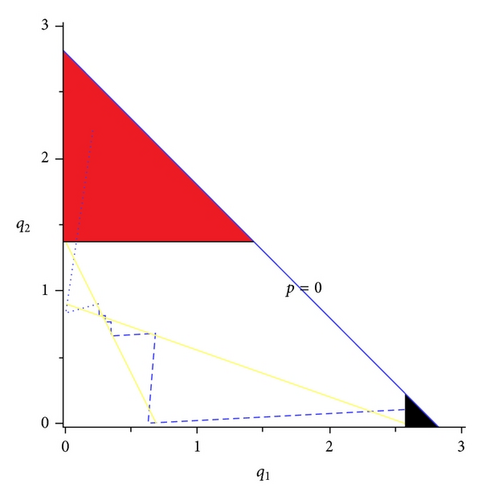
In addition, we note that in contrast with the standard Cournot game (γ = 1), under strategic uncertainty (γ < 1) it is more likely that the pessimistic (resp., optimistic) firm decides not to produce (resp., to produce) a positive quantity at a certain date (as shown in Figure 1).

Details are in the caption following the image — **Figure 1**
Open in figure viewer PowerPoint

Starting from the red (resp., black) region, the first iterate is (0, q₂), with q₂ > 0 (resp., (q₁, 0), with q₁ > 0). The yellow lines are the best reply curves of the two firms. The solid blue line represents points in which p = 0. The dotted and dashed blue lines represent trajectories that start from the red and black regions, respectively, and end up to the Nash equilibrium. Parameter set: a = 2.8, b = 1, c = 1, and γ = 0.7.

4. Dynamics under Limited Information

This section studies the dynamics of the Cournot model with strategic uncertainty by using an adjustment mechanism of production introduced by [17] in a model with continuous time and used by [18] in a model with discrete time. With regard to the information set of players, in this section we assume that both firms have limited information (no knowledge of the market demand) as in [11–14]. In order to overcome this informational lacuna, we assume that at any time t each player uses an adjustment mechanism based on local estimates of its own marginal CEU at time t (∂U/∂q) to determine production at time t + 1. The adjustment mechanism is as follows:

(19)

where α > 0 is a coefficient that captures the speed of adjustment of each firm’s quantity with respect to a marginal change in its marginal CEU and αq is the intensity of the reaction of each player. Therefore, in this case the pessimistic firm and the optimistic firm increase or decrease their production at time t + 1 depending on whether

and

are positive or negative, respectively. This type of adjustment mechanism implies that although players have incomplete information about demand and cost functions, they are able to get a correct estimate of their marginal CEU in the current period.

By using (4), (5), and (6), the two-dimensional system that characterises the dynamics of a Cournot duopoly, under strategic uncertainty and incomplete information is as follows:

(20)

From a mathematical point of view, map (20) is defined on the whole plane but for economic reasons only the dynamics that lie on set G = {(q₁, q₂) : q₁ ≥ 0, q₂ ≥ 0, q₁ + q₂ < a/b ∀ n} are meaningful (i.e., p > 0), where n is the number of iterations and the last inequality guarantees a positive value of the market price along the trajectory. We note that starting from initial conditions that lie on set D = {(q₁, q₂) : q₁ ≥ 0, q₂ ≥ 0, q₁ + q₂ ≤ a/b} does not guarantee that the dynamics remain on D for every iteration (i.e., (q₁, q₂) ∈ G). To avoid this problem, [13] and [19] introduce nonnegativity constraints on the mechanism of adjustment. This allows having well-defined trajectories by starting on whatever feasible initial condition from an economic point of view. By adapting this idea to the model under scrutiny we have that the map defined on set D becomes as follows:

(21)

Although in this paper we concentrate on the study of map (20), this does not represent a loss of generality, since it is possible to show that trajectories that exit from D coincide with trajectories of map (21) for which there exists a t^* such that for any t > t^* at least one of the two variables is zero; that is, one of the two firm exits from the market (see [13]).

4.1. Local Analysis

The fixed points of map (20) are obtained as nonnegative solutions of the algebraic system:

(22)

Thus, the stationary equilibria are the following:

, E₀ = (0,0), E₁ = (0, (a − c)/2b), and E₂ = ((aγ − c)/2bγ, 0).

The study of local stability of equilibrium solutions is based on the study of the Jacobian matrix:

(23)

evaluated at the fixed point.

Proposition 4. The fixed points E₀, E₁, and E₂ are unstable.

Proof. We have

(24)

The eigenvalues associated with (24) are λ₁ = 1 + α(γa − c) > 1 and λ₂ = 1 + α(a − c) > 1. Then, E₀ is a source:

(25)

The eigenvalues associated with (25) are λ₁ = 1 + [aγ − c(2 − γ)](α/2) > 1, where the sign of the inequality follows from Assumption 2, and λ₂ = 1 − α(a − c) < 1. Then, E₁ is a source or a saddle depending on the value of α:

(26)

The eigenvalues associated with (26) are λ₁ = 1 + (α[(2 − γ)a − c])/2 > 1, where the sign of the inequality follows from Assumption 2, and λ₂ = 1 + (c − aγ)α < 1. Then, E₂ is a source or a saddle depending on the value of α.

Proposition 5. The fixed point E^* is locally stable if and only if , where Dis (a) is defined in proof. For α = α_f, E^* undergoes a supercritical flip bifurcation. No other local bifurcations may arise around E^*.

Proof. The Jacobian matrix of map (20) evaluated at E^* is the following:

(27)

The trace and determinant associated with (27) are therefore given by

(28)

The local stability of Nash equilibrium is given by using Jury’s conditions; that is,

(29)

which for our system become

(30)

From condition a > a_low we have that second inequality in (30) is always verified; with regard to the third condition, we note that V₃ is a second-degree polynomial with respect to α. In addition, since 8a − 12c + 4cγ > 0 (in fact, a > a_low > (3 − γ)c/2) it follows that V₃ admits two positive roots α₁ and α₂, if the discriminant associated with the equation results to be positive. We now verify the sign of the discriminant. By simple calculations, we have that

(31)

This expression is quadratic in a and by a simple study we find that −γ³ + 6γ² − 8γ + 4 is always positive for any γ ∈ (0,1). Then, Dis(a) defines a concave function.

Now, since a > a_low, Dis(a_low) = (c(γ−1)(4−γ)/γ)² > 0 and Dis^′(a_low) = c(γ − 2) ²(γ − 1)(4 − γ)/γ > 0, then Dis(a) > 0 for any feasible value of a.

To sum up, V₃ > 0 for any α such that α < α₁∨α > α₂, where 0 < α₁ < α₂ and their explicit expressions are given by

(32)

With regard to the first condition in (30), we note that the sign of V₁ is given by the sign of

(33)

where v(α) is the first derivative of V₃. Then, v(α) = 0 for a value α_h ∈ (α₁, α₂), which corresponds to the minimum point of V₃. By considering the sign of the coefficients and inequalities involved, we have the result.

4.2. Critical Curves

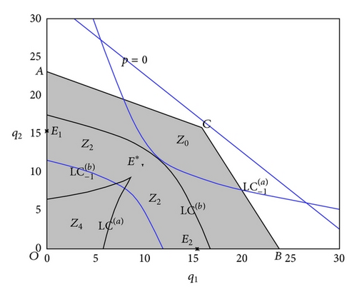
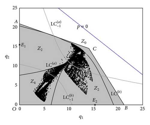
An important feature of map (20) is that it is a noninvertible endomorphism. In fact, for a given the rank-1 preimage (that is the backward iterate defined as ) may not exist or may be multivalued. In the specific case, if we want to compute (q₁, q₂) in terms of in (20) we have to solve a fourth-degree algebraic system that may have four, two, or no solutions. In a natural way, we are led to subdivide the plane in regions Z₀, Z₂, and Z₄ according to the number of such preimages (where the subscripts in Z indicate this number). A direct consequence of this fact is that if we let vary in the plane R², M₁, the number of the rank-1 preimages changes as the point crosses the boundary that separates these regions. Such boundaries are generally characterised by the existence of two coincident preimages. In this regard, by following [20] we introduce the definition of the critical curves. The critical curve of rank 1, denoted by LC is defined as the locus of points that have two (or more) coincident rank-1 preimages located on a set called LC₋₁. It is quite intuitive to interpret the set LC as the two-dimensional generalisation of the notion of critical value, local minimum or maximum, of a one-dimensional map, and LC₋₁ as the generalization of the notion of critical point (local extremum point). Arcs of LC separate the regions of the plane characterised by a different number of real preimages.

Since M₁ is a continuously differentiable map, LC₋₁ belongs to the locus of points where the Jacobian determinant of M₁ vanishes (i.e., the points where M₁ is not locally invertible). In our case,

(34)

and LC is the rank-1 image of LC₋₁ under M₁; that is, LC = M₁(LC₋₁).

From direct computation, we have that Det(J(q₁, q₂)) = 0 if and only if

(35)

It is easy to check that (35) is the equation of a hyperbola in the plane (q₁, q₂). Thus, LC₋₁ is formed by two branches, denoted by

and

. This implies that also LC and subsequent iterations of the critical curves may be seen as the union of two different branches. In Figure 2 we can read LC^(a) and LC^(b). Each branch of the critical curve LC separates the phase plane of M₁ into regions whose points have the same number of distinct rank-1 preimages. Specifically, LC^(b) separates region Z₀ from region Z₂, and LC^(a) separates region Z₂ from region Z₄. This allows us to study some global properties of the map and the evolution of basins of attraction and their qualitative changes (or bifurcations) as some parameters are varied.

4.3. Basins of Attraction

In this section, we describe the properties of the basins of attraction of map (20). We begin by studying the projection of the map on the Cartesian axes. For axes q₁ = 0 and q₂ = 0 we have, respectively,

(36)

(37)

We note that these equations are both conjugated to the logistic map z = μz(1 − z) through the transformation

(38)

with μ = 1 + α(a − c) for (36) and

(39)

with μ = 1 + α(aγ − c) for (37).

It follows that the dynamics on axes q₁ = 0 and q₂ = 0 can be obtained from the well-known behaviour of the standard logistic map by a homeomorphism (see [21]). In particular, (a) if 0 < α(a − c) < 3 (resp., 0 < α(aγ − c) < 3), then we can deduce that bounded trajectories along q₁ = 0 (resp., q₂ = 0) are generated if the initial conditions are taken inside the segment line ω₁ = [0, (1 + α(a − c))/2αb] (resp., ω₂ = [0, (1 + α(aγ − c))/2αbγ]; (b) from the computation of the eigenvalues of the cycles belonging to one of axes, we have that the direction transverse to the coordinate axes is always repelling; (c) initial conditions with or generate a divergent trajectory. From (a), (b), and (c) it follows that ω₁ and ω₂ and their preimages belong to the boundary of B(∞). In addition, under the conditions in (a), when the preimages belong to Z₀, we can show that B(∞) is given by the region outside the quadrilateral OABC with A(0, (1 + αa − αc)/2αb), B((1 + αaγ − αc)/2αbγ, 0), and where and so that the quadrilateral represents the region of trajectories that converge to a finite distance attractor that does not lie on the axes. Finally, from an economic point of view we note that, in order to preserve a positive value of the price inside the quadrilateral OABC, we have to impose the condition ; that is, a > 2(1 − αc)/αγ.

4.4. Global Analysis and Numerical Simulations

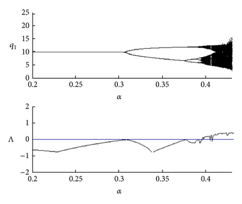
In this section we study the dynamic system M₁ for the following parameter values: a = 7.2, b = 0.22, c = 0.4, and γ = 0.9 and let α vary. Figures 3(a) and 3(b) show the existence of a period doubling cascade that (starting from the flip bifurcation value α = α_f≅0.3081) generates cyclic attractors of higher period until a global attractor is born.

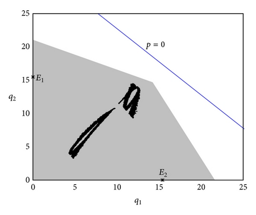
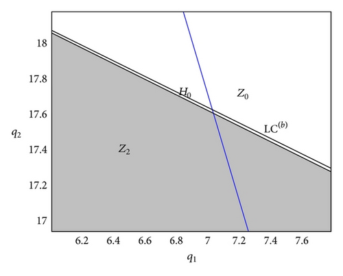
By increasing the value of α, we have an important topological change in the structure of the basins of attraction. In particular, when α≅0.4265 we have a tangency between LC^(b) and the upper side of the quadrilateral (the grey region in the figures). For higher values of α portions of the basin of attraction of the attractors on the axes enter Z₂ region (at least one of the firms exit the market). After the bifurcation (tangency), one main lake lies inside Z₂. Hence, the lake has further preimages which form smaller lakes within the grey region. These ones lie inside the quadrilateral in the region complement to Z₀. When α increases further, LC continues to move upwards, the portion H₀ grows up and then the holes become larger (see Figures 4(a) and 4(b)). At this stage it is really difficult to predict the long-term dynamics of the economic model, because slight changes in the initial conditions may lead to very different long-term outcomes (it is possible that only one firm produces or both firms produce but with erratic patterns). We note that the attractors located on the axes are not locally attracting. However, they attract a set of initial conditions with positive Lebesgue measure; that is, they are attractors à la Milnor (we recall that a closed invariant set A is a Milnor attractor if its stable set B(A) has positive Lebesgue measure (see [11] for details)). Finally, for α sufficiently large a contact bifurcation destroys the interior attractor.

5. Dynamics under Both Limited and Complete Information

In this section, we assume that firms adjust production period by period by using different mechanisms. In particular, the pessimistic firm has limited information and modifies production depending on the value of its own marginal profits, while the optimistic firm has complete information and static expectations (“best reply” dynamics). Given this type of heterogeneity and using (4) (pessimistic firm) and (7) (optimistic firm), the two-dimensional system that characterises the dynamics of the economy is now given by

(40)

which is defined on int (D).

Map (40) admits two fixed points: defined by (8) and . To guarantee that the unique Nash equilibrium of the game has economic meaning, we assume that the inequality a > c(2 − γ)/γ continues to be fulfilled. This condition also implies that the equilibrium values of profits and price are positive.

5.1. Local Analysis

The study of local stability of equilibrium solutions is based on the study of the Jacobian matrix of the dynamic system. The Jacobian matrix of map M₂ computed in a generic point has the following form:

(41)

The following propositions hold.

Proposition 6. The fixed point is unstable.

Proof. The Jacobian matrix of map (40) evaluated at is as follows

(42)

The eigenvalues associated with (42) are as follows: λ₀ = 0 and λ₁ = 1 + 1/2α[γ(a + c) − c] > 1.

Proposition 7. The fixed point E^* is locally stable if and only if . For , E^* undergoes a supercritical flip bifurcation. No other local bifurcations may arise around E^*.

Proof. The Jacobian matrix of map (40) evaluated at E^* is as follows:

(43)

The trace and determinant associated with (43) are therefore given by

(44)

The proof follows by using Jury’s conditions in (29), which are now given by

(45)

5.2. Global Dynamics

This section develops the global analysis of map (40). First of all, we note that if we relax the nonnegative constraints on variables q₁ and q₂, map (40) results to be invertible (i.e., given there exists one and only one (q₁, q₂)). However, map (40) is noninvertible with nonnegative constraints on q₁ and q₂. This can be ascertained by looking at Figure 5. From a global perspective, it is possible to identify regions on set D corresponding to which at least one of the best replies of the two firms is zero (Figure 5). It is important to note that the introduction of heterogeneity in the mechanism of adjustment between the two firms leads to different behaviours of the map along the Cartesian axes with respect to the model developed in Section 4. In particular, the axis q₁ = 0 is a trapping subset. In fact, when q₁ = 0 the subsequent iteration results to be (0, (a − c)/2b). In contrast, the axis q₂ = 0 does not have this property: the points that start on axis q₂ = 0 can lead to different fates (Figure 6(b)). Figure 5 shows that in the black region the subsequent iteration leads to a point (0, q₂), with q₂ > 0, while in the yellow region the subsequent iterate leads to a point (q₁, q₂) with q₁ > 0 and q₂ > 0. In the red region the subsequent iteration leads to (0,0) and finally the successive iterates will be located on the segment line OA.

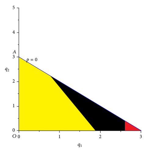
We note, however, that by starting from points that lie in the yellow region it is possible that the subsequent iteration continues to lie in the yellow region or, alternatively, it leads to either the red region or black region and the dynamics will definitely end up on the point (0, (a − c)/2b). In this case the side equilibrium is not locally attracting. However, it attracts a set of initial conditions with positive Lebesgue measure. From a mathematical point of view, these portions of the phase plane can be identified through the union of the preimages of any rank of the points in black and red regions.

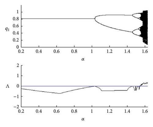
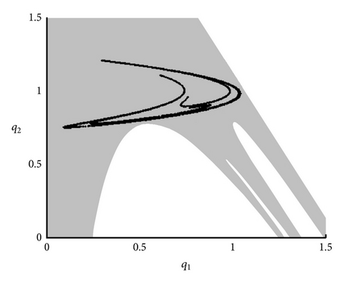
Analogously with map M₁, complex dynamics can be observed also for map M₂. Figures 6(a) and 6(b) show the bifurcation diagram and the corresponding Lyapunov exponent (Λ) for α by using the following parameter values: a = 3, b = 1, c = 0.5, and γ = 0.963. When α < 1.032, the interior fixed point is stable. Starting from , there exists a cascade of period-doubling bifurcations until the occurrence of a chaotic attractor, which is shown in Figure 6(b) that depicts the basin of attraction and the corresponding chaotic attractor for α = 1.61.

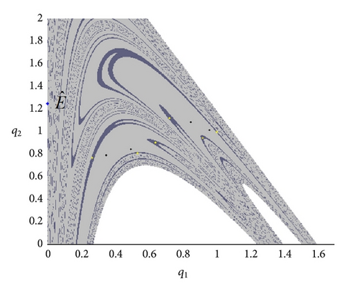
In addition, in the model with heterogeneous adjustment mechanisms we note that coexistence of interior attractors can occur by slightly reducing the value of α (this result is not usual in the nonlinear oligopoly literature with heterogeneous adjustment mechanisms [9, 10]). With this regard, Figure 7 shows that a cycle of period four (black points in the light-grey region) coexists with a cycle of period six (yellow points in the dark-grey region) when α = 1.498.

6. Conclusions

This paper developed a nonlinear Cournot duopoly to study the role of strategic uncertainty on the dynamics of the model economy. We characterised the local and global properties of a discrete two-dimensional map by considering that (1) both firms have complete information on the market demand and adjust production over time depending on past behaviours (static expectations, “best reply” dynamics); (2) both firms have incomplete information and production is adjusted over time by following a mechanism based on marginal profits; and (3) one firm has incomplete information and production decisions depend on marginal profits, and the rival has complete information with static expectations (mixed case). In cases 2 and 3 we showed the existence of complex phenomena such as chaotic attractors and coexistence of attractors. The different behaviour of the model depending on whether the adjustment mechanisms are homogeneous or heterogeneous is interesting from an economic point of view, because of the different long-term dynamics that can be observed. In particular, in the cases in which (a) both firms have incomplete information and the adjustment mechanism of production is homogeneous and (b) the information set available to firms and the adjustment mechanisms of production are mixed, there exists the possibility that at least one firm decides to exit from the market (i.e., to do not produce). This result does not hold when both firms have complete information on the market demand and production is based on the behaviour of the previous period.

Acknowledgments

The authors gratefully acknowledge that this work has been performed within the activity of the PRIN-2009 project “Local interactions and global dynamics in economics and finance: models and tools,” MIUR (Ministry of Education), Italy, and PRIN-2009 project “Structural change and growth,” MIUR, Italy. Numerical simulations have benefited from algorithms that can be found in http://dysess.wikispaces.com/. The authors also thank an anonymous reviewer for valuable comments. The usual disclaimer applies.

References

1 Bischi G. I., Chiarella C., Kopel M., and Szidarovszky F., Nonlinear Oligopolies. Stability and Bifurcations, 2010, Springer, Berlin, Germany, https://doi.org/10.1007/978-3-642-02106-0, MR2573046.
10.1007/978-3-642-02106-0
Google Scholar
2 Dow J. and Werlang S. R. D. C., Nash equilibrium under Knightian uncertainty: breaking down backward induction, Journal of Economic Theory. (1994) 64, no. 2, 305–324, https://doi.org/10.1006/jeth.1994.1071, MR1310256, ZBL0813.90132.
10.1006/jeth.1994.1071
Web of Science® Google Scholar
3 Eichberger J. and Kelsey D., Uncertainty and strategic interaction in economics, Discussion Papers, 1999, no. 99-26, Department of Economics, University of Birmingham.
Google Scholar
4 Eichberger J. and Kelsey D., Non-additive beliefs and strategic equilibria, Games and Economic Behavior. (2000) 30, no. 2, 183–215, https://doi.org/10.1006/game.1998.0724, MR1739571, ZBL0962.91002.
10.1006/game.1998.0724
Web of Science® Google Scholar
5 Marinacci M., Ambiguous games, Games and Economic Behavior. (2000) 31, no. 2, 191–219, https://doi.org/10.1006/game.1999.0739, MR1761312, ZBL0966.91002.
10.1006/game.1999.0739
Web of Science® Google Scholar
6 Chateauneuf A., Eichberger J., and Grant S., Choice under uncertainty with the best and worst in mind: neo-additive capacities, Journal of Economic Theory. (2007) 137, no. 1, 538–567, https://doi.org/10.1016/j.jet.2007.01.017, MR2888476, ZBL1132.91420.
10.1016/j.jet.2007.01.017
Web of Science® Google Scholar
7 Schmeidler D., Subjective probability and expected utility without additivity, Econometrica. (1989) 57, no. 3, 571–587, https://doi.org/10.2307/1911053, MR999273, ZBL0672.90011.
10.2307/1911053
Web of Science® Google Scholar
8 Fontini F., Cournot oligopoly under strategic uncertainty with optimistic and pessimistic firms, Metroeconomica. (2005) 56, no. 3, 318–333.
10.1111/j.1467-999X.2005.00219.x
Google Scholar
9 Agiza H. N. and Elsadany A. A., Chaotic dynamics in nonlinear duopoly game with heterogeneous players, Applied Mathematics and Computation. (2004) 149, no. 3, 843–860, https://doi.org/10.1016/S0096-3003(03)00190-5, MR2033167, ZBL1064.91027.
10.1016/S0096-3003(03)00190-5
Web of Science® Google Scholar
10 Tramontana F., Heterogeneous duopoly with isoelastic demand function, Economic Modelling. (2010) 27, no. 1, 350–357, 2-s2.0-71149121323, https://doi.org/10.1016/j.econmod.2009.09.014.
10.1016/j.econmod.2009.09.014
Web of Science® Google Scholar
11 Bischi G.-I., Stefanini L., and Gardini L., Synchronization, intermittency and critical curves in a duopoly game, Mathematics and Computers in Simulation. (1998) 44, no. 6, 559–585, https://doi.org/10.1016/S0378-4754(97)00100-6, MR1609542, ZBL1017.91500.
10.1016/S0378-4754(97)00100-6
Web of Science® Google Scholar
12 Bischi G.-I., Gallegati M., and Naimzada A., Symmetry-breaking bifurcations and representative firm in dynamic duopoly games, Annals of Operations Research. (1999) 89, no. 1–4, 253–272, https://doi.org/10.1023/A:1018931824853, MR1704056, ZBL0939.91017.
10.1023/A:1018931824853
Web of Science® Google Scholar
13 Fanti L., Gori L., and Sodini M., Nonlinear dynamics in a Cournot duopoly with relative profit delegation, Chaos, Solitons & Fractals. (2012) 45, no. 12, 1469–1478, https://doi.org/10.1016/j.chaos.2012.08.008, MR3000698, ZBL1258.91040.
10.1016/j.chaos.2012.08.008
Web of Science® Google Scholar
14 Fanti L., Gori L., Mammana C., and Michetti E., The dynamics of a Bertrand duopoly with differentiated products: synchronization, intermittency and global dynamics, Chaos, Solitons & Fractals. (2013) 52, 73–86, https://doi.org/10.1016/j.chaos.2013.04.002, MR3064184.
10.1016/j.chaos.2013.04.002
Web of Science® Google Scholar
15 Bischi G. I., Naimzada A. K., and Sbragia L., Oligopoly games with Local Monopolistic Approximation, Journal of Economic Behavior and Organization. (2007) 62, no. 3, 371–388, 2-s2.0-33846607851, https://doi.org/10.1016/j.jebo.2005.08.006.
10.1016/j.jebo.2005.08.006
Web of Science® Google Scholar
16 Puu T., Chaos in duopoly pricing, Chaos, Solitons & Fractals. (1991) 1, no. 6, 573–581.
10.1016/0960-0779(91)90045-B
Web of Science® Google Scholar
17 Dixit A., Comparative statics for oligopoly, International Economic Review. (1986) 27, no. 1, 107–122, https://doi.org/10.2307/2526609, MR829091, ZBL0584.90012.
10.2307/2526609
Web of Science® Google Scholar
18 Bischi G. I. and Naimzada A., J. A. Filar, V. Gaitsgory, and K. Mizukami, Global analysis of a dynamic duopoly game with bounded rationality, Advances in Dynamics Games and Application, 2000, 5, Birkhäuser, Boston, Mass, USA, 361–385.
10.1007/978-1-4612-1336-9_20
Google Scholar
19 Cánovas J. S., Puu T., and Ruíz M., The Cournot-Theocharis problem reconsidered, Chaos, Solitons and Fractals. (2008) 37, no. 4, 1025–1039, https://doi.org/10.1016/j.chaos.2006.09.081, MR2411530, ZBL1140.91444.
10.1016/j.chaos.2006.09.081
Web of Science® Google Scholar
20 Mira C., Gardini L., Barugola A., and Cathala J.-C., Chaotic Dynamics in Two-Dimensional Noninvertible Maps, 1996, World Scientific Publishing, Singapore, https://doi.org/10.1142/9789812798732, MR2001477.
10.1142/2252
Google Scholar
21 Devaney R. L., An Introduction to Chaotic Dynamical Systems, 1989, 2nd edition, Addison-Wesley, Redwood City, Calif, USA, MR1046376.
Google Scholar

Citing Literature

All articles

Nonlinear Dynamics in a Cournot Duopoly with Different Attitudes towards Strategic Uncertainty

Correction(s) for this article

Erratum to “Nonlinear Dynamics in a Cournot Duopoly with Different Attitudes towards Strategic Uncertainty”

Abstract

1. Introduction

2. The Model

3. Dynamics under Complete Information (“Best Reply” Dynamics)