Persistence and Nonpersistence of a Food Chain Model with Stochastic Perturbation
Abstract
We analyze a three species predator-prey chain model with stochastic perturbation. First, we show that this system has a unique positive solution and its pth moment is bounded. Then, we deduce conditions that the system is persistent in time average. After that, conditions for the system going to be extinction in probability are established. At last, numerical simulations are carried out to support our results.
1. Introduction
Recently, the dynamical relationship between predator-prey has been one of the dominant themes in both ecology and mathematical ecology due to its universal importance. Especially, the predator-prey chain model is the typical representative. Thereby it significantly changed the biology, the understanding of the existence, and development of the basic law and has made the model become a research hot spot. One of the most famous models for population dynamics is the Lotka-Volterra predator-prey system which has received plenty of attention and has been studied extensively; see [1–4]. Specially persistence and extinction of this model are interesting topics.
System (1) describes a three species predator-prey chain model in which the latter preys on the former. From a biological viewpoint, we not only require the positive solution of the system but also require its unexploded property in any finite time and stability.
Therefore, Lotka-Volterra predator-prey chain models in random environments are becoming more and more popular. Ji et al. [14, 15] investigated the asymptotic behavior of the stochastic predator-prey system with perturbation. Liu and Chen introduced periodic constant impulsive immigration of predator into predator-prey system and gave conditions for the system to be extinct and permanence. Polansky [17] and Barra et al. [18] have given some special systems of their invariant distribution. After that, Gard [5] analysed that under some conditions the stochastic food chain model exists an invariant distribution. However, seldom people study the persistent and nonpersistent of the food chain model with stochastic perturbation.
The aim of this paper is to discuss the long time behavior of system (3). We have mentioned that is the positive equilibrium of system (1). But, when it suffers stochastic perturbations, there is no positive equilibrium. Hence, it is impossible that the solution of system (3) will tend to a fixed point. In this paper, we show that system (3) is persistent in time average. Furthermore, under certain conditions, we prove that the population of system (3) will die out in probability which will not happen in deterministic system and could reveal that large white noise may lead to extinction.
The rest of this paper is organized as follows. In Section 2, we show that there is a unique nonnegative solution of system (3), and its pth moment is bounded. In Section 3, we show that system (3) is persistent in time average. While in Section 4, we consider three situations when the population of the system will be extinction. In Section 5, numerical simulations are carried out to support our results.
Throughout this paper, unless otherwise specified, let (Ω, {ℱt} t≥0, P) be a complete probability space with a filtration {ℱt} t≥0 satisfying the usual conditions (i.e., it is right continuous and ℱ0 contains all P-null sets). Let denote the positive cone of R3; namely, , .
2. Existence and Uniqueness of the Nonnegative Solution
To investigate the dynamical behavior, the first concern thing is whether the solution is global existence. Moreover, for a population model, whether the solution is nonnegative is also considered. Hence, in this section, we show that the solution of system (3) is global and nonnegative. As we have known, in order for a stochastic differential equation to have a unique global (i.e., no explosion at a finite time) solution with any given initial value, the coefficients of the equation are generally required to satisfy the linear growth condition and local Lipschitz condition (see, e.g., [19]). It is easy to see that the coefficients of system (3) are locally Lipschitz continuous, so system (3) has a local solution. By Lyapunov analysis method, we show the global existence of this solution.
Theorem 1. For any given initial value , system (3) has a unique global positive solution x(t) = (x1(t), x2(t), x3(t)) for all t ≥ 0 with probability one.
Proof. It is clear that the coefficients of system (3) are locally Lipschitz continuous for the given initial value . So there is a unique local solution x(t) on t ∈ [0, τe), where τe is the explosion time (see, e.g., [19]). To show that this solution is global, we need to show that τe = ∞ a.s. Let m0 ≥ 1 be sufficiently large so that each component of x0 all lies within the interval [1/m0, m0]. For each integer m ≥ m0, define the stopping time:
Theorem 2. Let x(t) = (x1(t), x2(t), and let x3(t)) be the solution of system (3) with any given initial value , then there exists a positive constant K(p) such that
Proof. Let y(t) = b32b21x1(t) + b32b12x2(t) + b23b12x3(t); then
3. Persistent in Time Average
There is no equilibrium of system (3). Hence we cannot show the permanence of the system by proving the stability of the positive equilibrium as the deterministic system. In this section we first show that this system is persistent in mean. Before we give the result, we should do some prepared work.
L. S. Chen and J. Chen in [20] proposed the definition of persistence in mean for the deterministic system. Here, we also use this definition for the stochastic system.
Definition 3. System (3) is said to be persistent in mean, if
Lemma 4 (see [21], Lemma 17.)Let f ∈ C([0, +∞) × Ω, (0, +∞)) and F ∈ C([0, +∞) × Ω, R). If there exist positive constants λ0, λ, such that
From Lemma 4, it is easy to see that we could get Lemmas 5 and 6 with the same method.
Lemma 5. Let f ∈ C([0, +∞) × Ω, (0, +∞)) and F ∈ C([0, +∞) × Ω, R). If there exist positive constants λ0, λ, such that
Lemma 6. Let f ∈ C([0, +∞) × Ω, (0, +∞)) and F ∈ C([0, +∞) × Ω, R). If there exist positive constants λ0, λ, such that
From the stochastic comparison theorem [11], it is easy to get the following result.
Lemma 7. Let be a solution of system (3) with x(0) = (x1(0), x2(0), x3(0)). Then one has
Assumption 8. Consider
Lemma 9. If Assumption 8 is satisfied, the solution Φ(t) of system (32) with any initial value has the following property:
Proof. From the result in [14] and Assumption 8 being satisfied, we know
From this, together with Lemmas 7 and 9, the following result is obviously true.
Theorem 10. If Assumption 8 is satisfied, the solution x(t) of system (3) with any initial value has the following property:
Above all, we could get.
Theorem 11. If Assumption 8 is satisfied, the the solution x(t) of system (3) with any initial value has the following property:
Proof. From system (3), such that
4. Nonpersistence
In this section, we show the situation when the population of system (3) will be extinction in three cases.
Case 1 (r1 < 0). According to Itô′s formula, the first population of system (25) is changed into
Case 2 (r1 > 0, r1 − (b11/b21)r2 < 0). It is clear that from the proof section of Case 1, we get
Case 3 (r1 − (b11/b21)r2 − ((b11b22 + b12b21)/b21b32)r3 < 0). It is clear that
Theorem 12. Let x(t) be the solution of system (3) with any initial value . Then
(1) if r1 < 0, then
(2) if r1 > 0, r1 − (b11/b21)r2 < 0, then
(3) if r1 − (b11/b21)r2 − ((b11b22 + b12b21)/b21b32)r3 < 0, then
5. Numerical Simulation


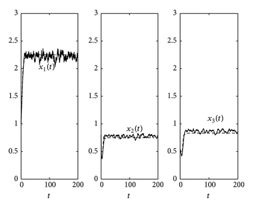
In Figure 1, when the noise is small, choosing parameters satisfying the condition of Theorem 10, the solution of system (3) will persist in time average.
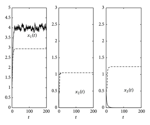
In Figure 2, we observe case (3) in Theorem 12 and choose parameters r1 > 0, r1 − (b11/b21)r2 < 0. As Theorem 12 indicated that two predators will die out in probability. The prey solution of system (3) will persist in time average.
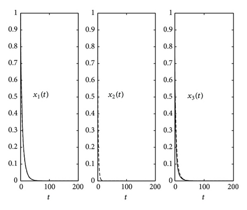
In Figure 3, we observe case (1) in Theorem 12 and choose parameters r1 < 0. As Theorem 12 indicated that not only predators but also prey will die out in probability when the noise of the prey is large, and it does not happen in the deterministic system.
Acknowledgments
The work was supported by the Ministry of Education of China (no. 109051), the Ph.D. Programs Foundation of Ministry of China (no. 200918), and NSFC of China (no. 11371085), Natural Science Foundation of Jilin Province of China (no. 201115133).


