Measuring Non-Gaussianity by Phi-Transformed and Fuzzy Histograms
Abstract
Independent component analysis (ICA) is an essential building block for data analysis in many applications. Selecting the truly meaningful components from the result of an ICA algorithm, or comparing the results of different algorithms, however, is nontrivial problems. We introduce a very general technique for evaluating ICA results rooted in information-theoretic model selection. The basic idea is to exploit the natural link between non-Gaussianity and data compression: the better the data transformation represented by one or several ICs improves the effectiveness of data compression, the higher is the relevance of the ICs. We propose two different methods which allow an efficient data compression of non-Gaussian signals: Phi-transformed histograms and fuzzy histograms. In an extensive experimental evaluation, we demonstrate that our novel information-theoretic measures robustly select non-Gaussian components from data in a fully automatic way, that is, without requiring any restrictive assumptions or thresholds.
1. Introduction
Independent component analysis (ICA) is a powerful technique for signal demixing and data analysis in numerous applications. For example, in neuroscience, ICA is essential for the analysis of functional magnetic resonance imaging (fMRI) data and electroencephalograms (EEGs). The function of the human brain is very complex and can be only imaged at a very coarse spatial resolution. Millions of nerve cells are contained in a single voxel of fMRI data. The neural activity is indirectly measured by the so-called BOLD-effect, that is, by the increased supply of active regions with oxygenated blood. In EEG, the brain function can be directly measured by the voltage fluctuations resulting from ionic current flows within the neurons. The spacial resolution of EEG, however, is even much lower than that of fMRI. Usually, an EEG is recorded using an array of 64 electrodes distributed over the scalp. Often, the purpose of acquiring fMRI or EEG data is obtaing a better understanding of brain function while the subject is performing some task. An example for such an experiment is to show subjects images while they are in the scanner to study the processing of visual stimuli, see Section 4.1.4. Recent results in neuroscience, for example [1], confirm the organization of the human brain into distinct functional modules. During task processing, some functional modules are actively contributing to the task. However, many other modules are also active but not involved into task-specific activities. Due to the low resolution of fMRI and EEG data, we observe a partial volume effect: the signal at one particular voxel or electrode consists of task-related activities, nontask-related activities, and a lot of noise. ICA is a powerful tool for signal demixing and, therefore, in principle very suitable to reconstruct the interesting task-related activity.
Many ICA algorithms use the non-Gaussianity as implicit or explicit optimization goal. The rationale behind this decision is due to a reversion of the central limit theorem: the sum of a sufficiently large number of independent random variables, each with finite mean and variance, will approximate a normal distribution. Therefore, an algorithm for the demixing of signals has to optimize for non-Gaussianity in order to obtain the original signals. We adopt this idea in this paper and define a data compression method which yields a high compression rate exactly if the data distribution is far away from Gaussianity and no compression in the data distribution is exactly gaussian.
However, the evaluation and interpretation of the result of ICA is often difficult for two major reasons. First, most ICA algorithms always yield a result, even if the underlying assumption (e.g., non-Gaussianity for the algorithm FastICA [2]) is unfulfilled. Thus, many ICA algorithms extract as many independent sources as there are mixed signals in the dataset, no matter how many of them really fulfill the underlying assumption. Second, ICA has no unique and natural evaluation criterion to assess the relevance or strength of the detected result (like, e.g., the variance criterion for principle component analysis (PCA)). Different ICA algorithms use different objective functions, and to select one of them as an overall objective, or neutral criterion would give unjustified preference to the result of that specific algorithm. Moreover, if the user is interested in comparing an ICA result to completely different modeling techniques like PCA, regression, mixture models, and so forth, these ICA-internal criteria are obviously unsuitable. Depending on the actual intension of the user, different model selection criteria for ICA might be appropriate. In this paper, we investigate the compressibility of the data as a more neutral criterion for the quality of single component or the overall ICA result.
2. Related Work
2.1. Model Selection for ICA
Model selection for ICA or automatically identifying the most interesting components is an active research question. Perhaps the most widely used options for model selection are measures like Kurtosis, Skewness, and approximations of neg-entropy [3]. However, these measures are also applied as optimization criteria by some ICA algorithms. Thus, a comparison of the results across algorithms is impossible. Moreover, these measures are very sensitive with respect to noise points and single outliers.
In [4], Rasmussen et al. propose an approach for model selection of epoched EEG signals. In their model order selection procedure, the data set is split into two sets, training- and test set, to ensure an unbiased measure of generalization. With each model hypothesis, the negative logarithm of the likelihood function is then calculated using a probabilistic framework on the training and test set. The model having minimal generalization error is selected. This approach, however, is based on certain assumptions about source autocorrelation and tends to be sensitive to noise.
The most common method for model order selection is based on principal component analysis (PCA) of the data covariance matrix, which is proposed by Hyvärinen et al. [3]. The choice of number of sources to be selected is based on the number of dominant eigenvalues which significantly contribute to the total variance. This approach is fast and simple to implement, however, it suffers from a number of problems, for example, an inaccurate eigenvalue decomposition of the data covariance matrix in the noise-free case with fewer numbers of sources than sensors and sensitivity to noise. Moreover, there are no reasons to say that the subspace spanned by dominant principal components contains the source of interest [5]. Another approach proposed by James and Hesse [5] is to do the step-wise extraction of the sources until it reaches a predefined accuracy. However, the choice of reasonable accuracy level is also one drawback of this algorithm.
Related to model selection but still a different problem is the reliability of ICA results. The widely used iterative fix-point algorithm FastIca [6] converges towards different local optima of the optimization surface. The technique Icasso [7] combines Bootstrapping with a visualization to allow the user to investigate the relationship between different ICA results. Reliable results can be easily identified as dense clusters in the visualization. However, no information on the quality of the results is provided, which is the major focus of our work. Similar to Icasso, Meinecke et al. [8] proposed a resampling method to assess the quality ICA results by computing the stability of the independent subspaces. First, they create surrogate datasets by randomly selecting independent components from an ICA decomposition and apply the ICA algorithm for each of the surrogate data sets. Then, they separate the data space into one or multidimensional subspaces by their block structure and compute the uncertainty for each subspace. This proposed reliability estimation can be used to choose the appropriate BSS-model, to enhance the separation performance and, most importantly, to flag components which have a physical meaning.
2.2. Minimum Description Length for Model Selection
The minimum description length (MDL) principle is based on the simple idea that the best model to describe the data is one with the overall shortest description of the data and model itself, and it is essentially the same as Occam′s razor.
The MDL principle has been successfully applied for model selection for a large variety of tasks, ranging from linear regression [9], image segmentation [10] to polyhedral surface models [11].
In data mining, the MDL principle has recently attracted some attention enabling parameter-free algorithms to graph mining [12], clustering, for example [13–15], and outlier detection [16]. Sun et al. [12] proposed GraphScope, a parameter-free technique to mine information from streams of graphs. This technique used MDL to decide how and when to form and modify communities automatically. Böhm et al. [15] proposed OCI, a novel fully automatic algorithm to clustering non-Gaussian data with outliers, based on MDL to control the splitting, filtering, and merging phase in a parameter-free and very efficient top-down clustering approach. CoCo [16], a technique for parameter-free outlier detection, is based on the ideas of data compression and coding costs. CoCo used MDL to define an intuitive outlier factor together with a novel algorithm for outlier detection. This technique is parameter free and can be applied to a wide range of data distributions. OCI combines local ICA with clustering and outlier filtering. Related to this idea, in [17], Gruber et al. propose an approach for automated image de-noising combining local PCA or ICA with model selection by MDL.
In this paper, we propose a model selection criterion based on the MDL principle suitable for measuring the quality of single components as well as complete ICA results.
3. Independent Component Analysis and Data Compression
One of the fundamental assumptions of many important ICA algorithms is that independent sources can be found by searching for maximal non-Gaussian directions in the data space. Non-Gaussianity leads to a decrease in entropy, and therefore, to a potential improvement of the efficiency of data compression. In principle, the achievable compression rate of a dataset, after ICA, is higher compared to the original dataset. The principle of minimum description length (MDL) uses the probability P(x) of a data object x to represent it according to Huffman coding. Huffman coding gives a lower bound for the compression rate of a data set D achievable by any concrete coding scheme, as follows: ∑x∈D − log 2(P(x)). If x is taken from a continuous domain (e.g., the vector space ℛd for the blind source separation of a number d of signals), the relative probability given by a probability density function p(x) is applied instead of the absolute probability. The relative and absolute log-likelihoods (which could be obtained by discretizing x) are identical up to a constant value which can be safely ignored, as we discuss in detail in Section 3.1. For a complete description of the dataset (allowing decompression), the parameters of the probability density function (PDF) such as mean and variance for Gaussian PDFs need to be coded and their code lengths added to the negative log-likelihood of the data. We call this term the code book. For each parameter, a number of bits equal to (1/2)log 2(n) where n is the number of objects in D, is required, as fundamental results from information theory have proven [18]. Intuitively, the term (1/2)log 2(n) reflects the fact that the parameters need to be coded more precisely when a higher number n of data objects is modeled by the PDF. The MDL principle is often applied for model selection of parametric models like Gaussians, or Gaussian mixture models (GMMs). Gaussian mixture models vary in the model complexity, that is, the number of parameters needed for modeling. MDL-based techniques are well able to compare models of different complexity. The main purpose of the code book is to punish complexity in order to avoid overly complex, over-fitted models (like a GMM having one component exactly at the position of each data object: such a model would yield a minimal Huffman coding, but also a maximal code-book length). By the two concepts, Huffman coding using the negative log-likelihood of a PDF and the code-book for the parameters of the PDF, the principle of MDL provides a very general framework which allows the comparison of very different modeling techniques like principal component analysis (based on a Gaussian PDF model), clustering [13], regression [19] for continuous domains, but, in principle, also for discrete or mixed domains. At the same time, model complexity is punished and, therefore, overfitting avoided. Related criteria for general model selection include, for example, the Bayesian information criterion and the Aikake information criterion. However, these criteria are not adapted to the ICA model. In the following section, we discuss how to apply the MDL principle in the context of ICA.
3.1. General Idea of the Minimum Description Length Principle
We simply have to observe that (1) the resolution is not implicitly changed by any transformations of the dataset (like, e.g., a linear scaling α · x of the data objects) and (2) that ignoring the term might lead to negative values of NLLHf(D) (so we partly lose the nice intuition of a number of bits encoding the data objects, and particularly that 0 is a lower limit of this amount of information).
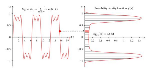
The principle of coding a signal with a pdf f(x) is visualized in Figure 1 where a signal (a superposition of three sinuses) is coded. To represent one given point of the signal (at t = 15.5), we should actually use a discretization of x as indicated in the right part of the diagram to obtain an actual code length for the value x. However, we can also directly use the negative log-likelihood of the value x with the above-mentioned implications.
We will in the following sections propose nonparametric methods which are both related to histograms. Therefore, the number of parameters in principle corresponds to the number of bins. We do not use histograms directly since our goal is to code the signals in a way that punishes the Gaussianity and rewards the non-Gaussianity. Thus, we propose two different methods which modify the histogram concept in a suitable way.
3.2. Phi-Transformed Histograms
Techniques like [15] or [20] successfully use the exponential power distribution (EPD), a generalized distribution function including Gaussian, Laplacian, uniform, and many other distribution functions for assessing the ICA result using MDL. The reduced entropy of non-Gaussian projections in the data allows a higher compression rate and thus favors a good ICA result. However, the selection of EPD is overly restrictive. For instance, multimodal and asymmetric distributions cannot be well represented by EPD but are highly relevant to ICA. In the following, we describe an alternative representation of the PDF which is efficient if (and only if) the data is considerably different from Gaussian. Besides the non-Gaussianity, we have no additional assumption (like for instance EPD) on the data. To achieve this, we tentatively assume Gaussianity in each signal of length n and transform the assumed Gaussian distribution into a uniform distribution in the interval (0,1) by applying the Gaussian cumulative distribution function Φ((x − μ)/σ) (the Φ-transformation) to each signal of the data representation to be tested (e.g., after projection on the independent components). Then, the resulting distribution is represented by a histogram (H1, …, Hb) with a number b of equidistant bins where b is optimized as we will show later. Hj(1 ≤ j ≤ b) is the number of objects falling in the corresponding half open interval [(j − 1)/b, j/b). If the signal is Gaussian indeed, then the signals after Φ-transformation will be uniform and the histogram bins will be (more or less) uniformly filled. Therefore, a trivial histogram with only one bin will in this case yield the best coding cost (and thus, no real data compression comes into effect). The Φ-transformation itself causes a change of the coding cost which is equivalent to the entropy of the Gaussian distribution function, as we show in as follows.
As introduced in Section 3, the first two terms represent the negative log-likelihood of the data given the histogram. The first corresponds to the entropy of the histogram, and the second term, stemming from casting the histogram into a PDF, has also the following intuition: when coding the same data with a varying number of histogram bins, the resulting log-likelihoods are based on different basic resolutions of the data space (a grid with a number b of partitions). Although the choice of a particular basic resolution is irrelevant for the end-result, for comparability, all alternative solutions must be based on a common resolution. We choose g = 1 as basic resolution, and subtract for each object the number of bits by which we know the position of the object more precisely than in the basic resolution. The trivial histogram having b = 1 represents the case where the data is assumed to be Gaussian: since the Gaussian cumulative distribution function Φ((x − μ)/σ) has been applied to the data, Gaussian data are transformed into uniform data, and our histograms have an implicit assumption of uniformity inside each bin. Therefore, we call it offset cost because it stands for coding the position of a value inside a histogram bin. If some choice of b ≠ 1 leads to smaller CLRG(D, b), we have evidence that the signal is different from Gaussian. It is easy to see that in the case b = 1 the code length is CLRG(D, b) = PRE, which is a consequence of our definition of the offset cost. Therefore, we call our cost function code length relative to Gaussianity, (CLRG). If no choice that b ≠ 1 leads to CLRG(D, b) < PRE, then either the data is truly Gaussian or the number of data objects is not high enough to give evidence for non-Gaussianity. In the latter case, we use Gaussianity as the safe default-assumption. The third term is the cost required for the code book: to completely describe b histogram bins it is sufficient to use b − 1 codewords since the remaining probability is implicitly specified. The last term, PRE is for preprocessing, that is, taking the Φ-transform into account.
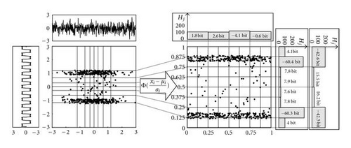
Figure 2 gives an overview and example of our method. On the left side, the result of an ICA run is depicted which has successfully separated a number d = 2 of signals (each having n = 500 points). The corresponding scatter-plot shows a Gaussian signal on the x-axis, a rectangular signal on the y-axis (note that the corresponding signal plots on the axes are actually transposed for better visibility). On the right side, we see the result after applying the Gaussian CDF. Some histograms with different resolutions are also shown. On the x-axis, the histogram with b = 4 bins is approximately uniformly filled (like also most other histograms with a different selection of b). Consequently, only a very small number of bits is saved compared to Gaussianity (e.g., only 4.1 bits for the complete signal part falling in the third bin H3) by applying this histogram as PDF in Huffman coding (here, the cost per bin are reported including log-likelihood and offset-cost). The overall saving of 0.29 bit are contrasted by a code-book length of (3/2)log 2n = 13.4, so the histogram representation does not pay off. In contrast, the two histograms on the y-axis do pay off, since for b = 8, we have overall savings over Gaussianity of 81.3 bit by Huffman coding, but only (7/2)log 2n = 31.4 bits of codebook.
3.2.1. An Optimization Heuristic for the Histogram Resolution
We need to optimize b individually for each signal such that the overall coding cost CLRG(D, b) is minimized. As an efficient and effective heuristic, we propose to only consider histogram resolutions where b is a power of 2. This is time efficient since the number of alternative results is logarithmic in n (as we will show), and the next coarser histogram can be intelligently gained from the previous. In addition, the strategy is effective since a sufficient number of alternative results is examined.
3.3. Fuzzy Histograms
Often histograms are not a good description of data since they define a discontinuous function whereas the original data distribution often corresponds to a continuous function. Since we want to focus on non-Gaussianity without any other assumption on the underlying distribution function, a good alternative to histograms is fuzzy histograms. In statistics, often kernel density estimators (KDEs) are applied in cases where a continuous representation of the distribution function is needed. However, KDEs require a number of parameters which is higher than the number of objects, and, therefore, KDEs are not suitable for our philosophy of compressing the dataset according to the defined distribution function (although other information-theoretic KDEs exist). Therefore, we apply the simpler fuzzy histograms which extend histograms as follows.
which is continuous (as it is a sum of continuous functions) and integrates to 1 (as all wi sum up to one and each kernel function integrates to 1).
That means that we set the initial slope m = (μb − μ1)/b and t = μ1 − m.
These steps starting from evaluation (22) are repeated until convergence.
4. Experiments
This section contains an extensive experimental evaluation. We start by a proof of concept demonstrating the benefits of information-theoretic model selection for ICA over established model selection criteria such as kurtosis in Section 4.1. Since in these experiments phi-transformed histograms and equidistant Gaussian Mixture Models perform very similar, for space limitations, we only show the results of phi-transformed histograms. In Section 4.2, we discuss the two possibilities of estimating the code length relative to Gaussianity.
4.1. Proof of Concept: Information-Theoretic Model Selection for ICA
4.1.1. Selection of the Relevant Dimensions
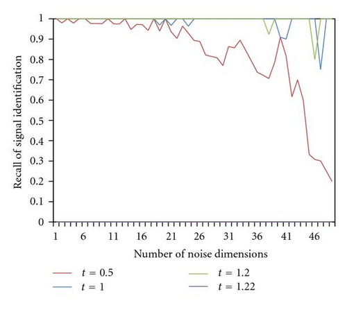
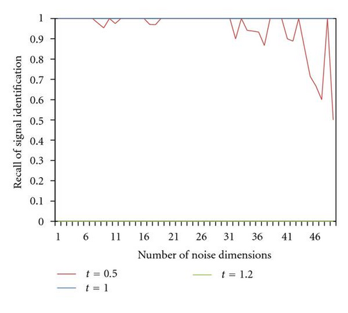
Which ICs truly represent meaningful signals? Measures like kurtosis, skewness, and other approximations of neg-entropy are often used for selecting the relevant ICs but need to be suitably thresholded, which is a nontrivial task. Figures 3(a) and 3(b) display the recall of signal identification for a dataset consisting of highly non-Gaussian saw-tooth signals and a varying number of noise dimensions for various thresholds of kurtosis. Kurtosis is measured as the absolute deviation from Gaussianity. The recall of signal identification is defined as the number of signals which have been correctly identified by the selection criterion divided by the overall number of signals. Figure 3(a) displays the results for various thresholds on a dataset with 200 samples. For this signal length, a threshold of t = 1.2 offers the best recall in signal identification for various numbers of noise dimensions. A slightly higher threshold of 1.22 leads to a complete break down in recall to 0, which implies that all noise signals are rated as non-Gaussian by kurtosis. For the dataset of 500 samples, however, t = 1.0 is a suitable threshold and for t = 1.2, we can observe a complete breakdown in recall. Even on these synthetic examples with a very clear distinction into highly non-Gaussian signals and Gaussian noise, the range for suitable thresholding is very narrow. Moreover, the threshold depends on the signal length and of course strongly on the type of the particular signal. A reasonable approach to select a suitable threshold is to try out a wide range of candidate thresholds and to select the threshold maximizing the area under ROC. For most of our example datasets with 200 samples, a threshold of t = 1.2 maximizes the area under ROC. For the datasets with 20 to 36 noise dimensions, this threshold yields a perfect result with an area under ROC of 1.0. For 500 samples, however, a lower threshold is preferable on most datasets. Supported by information theory, CLRG automatically identifies the relevant dimensions without requiring any parameters or thresholds. For all examples, CLRG identifies the relevant dimensions as those dimensions allowing data compression with a precision and a recall of 100%.
4.1.2. Stable Estimation of the IC Quality
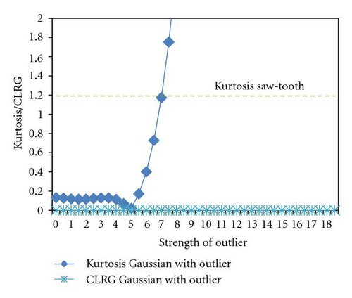
Commonly used approximations of neg-entropy are sensitive to single outliers. Outliers may cause an overestimation of the quality of the IC. CLRG is an outlier-robust measure for the interestingness of a signal. Figure 3(c) displays the influence of one single outlier on the kurtosis (displayed in terms of deviation from Gaussian) and CLRG of a Gaussian noise signal with 500 samples with respect to various outlier strengths (displayed in units of standard deviation). For reference, also the kurtosis of a highly non-Gaussian saw-tooth signal is displayed with a dotted line. Already for moderate outlier strength, the estimation of kurtosis becomes unstable. In case of a strong single outlier, kurtosis severely overestimates the interestingness of the signal. CLRG is not sensitive with respect to single outliers: even for strongest outliers, the noise signal is scored as not interesting with a CLRG of zero. For comparison, the saw-tooth curve allows an effective data compression with a CLRG of −553.
4.1.3. Comparing ICA Results
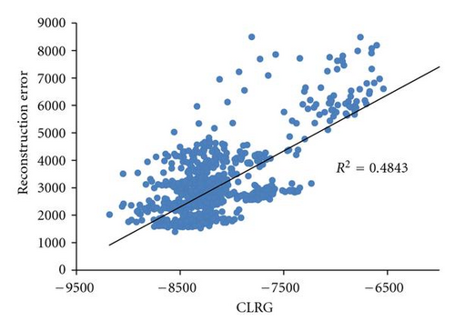
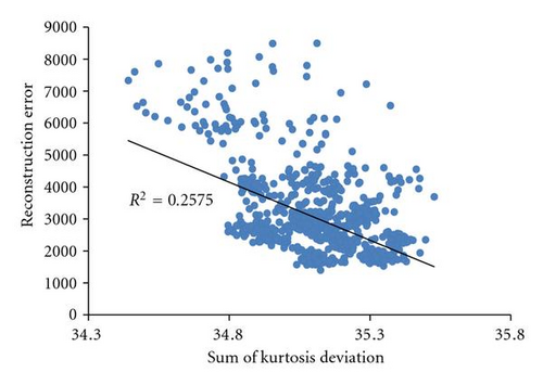
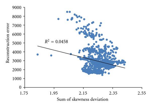
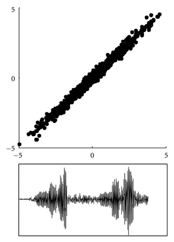
CLRG is a very general criterion for assessing the quality of ICA results which does not rely on any assumptions specific to certain algorithms. In this experiment, we compare CLRG to kurtosis and skewness on the benchmark dataset acspeec16 form ICALAB (http://www.bsp.brain.riken.go.jp/ICALAB/ICALABSignalProc/benchmarks/). This dataset consists of 16 speech signals which we mixed with a uniform random mixing matrix. Figure 4 displays 1,000 results of FastIca [2] generated with the nonlinearity tanh and different random starting conditions. For each result, we computed the reconstruction error as the sum of squared deviations of the ICs found by FastIca to the original source signals. For each IC, we used the best matching source signal (corrected for sign ambiguity) and summed up the squared deviations. Figure 4(a) shows that CLRG correlates best with the reconstruction error. In particular, ICA results with a low reconstruction error also allow effective data compression. For comparison, we computed the sum of kurtosis deviations and the sum of skewness deviations from Gaussianity. Kurtosis and even more skewness show only a slight correlation with the reconstruction error. As an example, Figure 5(a) shows the first extracted IC from the result best scored by CLRG and the corresponding IC (Figure 5(b)) from the result best scored by kurtosis. For each of the two ICs the scatter plots with the original signal are displayed. Obviously, the left IC better matches the true signal than the right IC resulting in a lower reconstruction error.

4.1.4. Selecting Relevant Components from fMRI Data
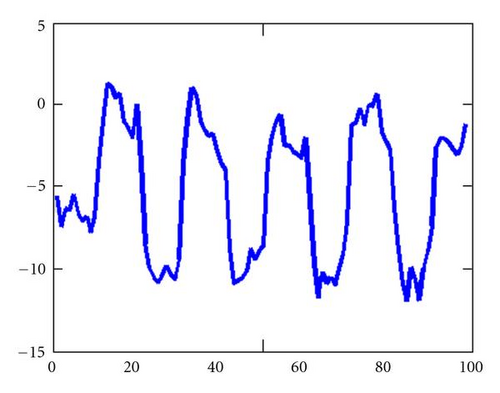
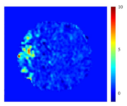
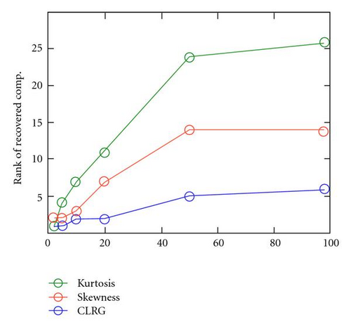
Functional magnetic resonance imaging (fMRI) yields time series of 3-d volume images allowing to study the brain activity, usually while the subject is performing some task. In this experiment, a subject has been visually stimulated in a block-design by alternately displaying a checkerboard stimulus and a central fixation point on a dark background as control condition [21]. fMRI data with 98 images (TR/TE = 3000/60 msec) were acquired with five stimulation and rest periods having each a duration of 30 s. After standard preprocessing, the dimensionality has been reduced with PCA. FastIca has been applied to extract the task-related component. Figure 6(a) displays an example component with strong correlation to the experimental paradigm. This component is localized in the visual cortex which is responsible for processing photic stimuli, see Figure 6(b). We compared CLRG to kurtosis and skewness with respect to their scoring of the task-related component. In particular, we performed PCA reductions with varying dimensionality and identified the component with the strongest correlation to the stimulus protocol. Figure 6(c) shows that CLRG scores the task-related component much better than skewness and kurtosis. Regardless of the dimensionality, the task-related component is always among the top-ranked components by CLRG, in most cases among the top 3 to 5. By kurtosis and skewness, the interest of task-related component often rated close to the average.
4.2. Discussion of CLRG Estimation Techniques
Phi-transformed histograms and equidistant Gaussian mixture models represent different possibilities to estimate the code length relative to Gaussianity (CLRG). As elaborated in Section 3, to estimate the code length in bits, we need a probability density function (PDF) and the two variants differ in the way the PDF is defined. The major benefit of equidistant Gaussian mixture models over Phi-transformed histograms is that the PDF is defined by a continuous function which tends to represent some signals better than phi-transformed histograms. A better representation of the non-Gaussian characteristics of a signal results in more effective data compression expressed by a lower CLRG.
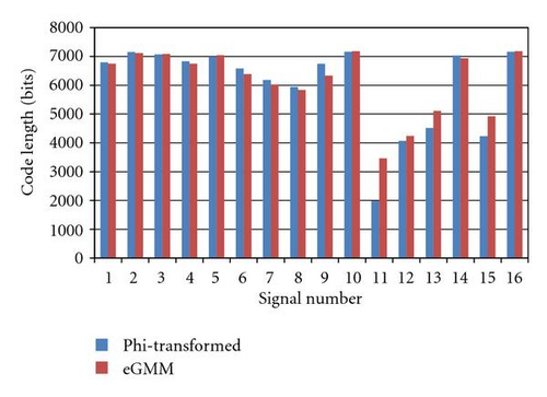
Figure 7 provides a comparison of phi-transformed histograms and equidistant Gaussian mixture models (eGMMs) regarding the CLRG estimated for the 16 signals of the aspeech16 dataset. For most signals, the CLRG estimated by both variants is very similar, for example, signals number 1 to 3, 10, and 16. Eight signals can be most effectively compressed using phi-transformed histograms, most evidently signals number 11 to 13. The other eight signals can be most effectively compressed using eGMM. In average on the aspeech16 dataset, the average CLRG 6,028 bits for phi-transformed histograms, 6,148 bits for eGMM.
We found similar results on other benchmark datasets also available at the ICALAB website: the 19 signals of the eeg19 dataset tend to be better represented by eGMM with an average CLRG of 17,691 (11 signals best represented by eGMM) followed by phi-transformed histograms with an average CLRG of 17,807 (8 signals best represented by phi-transformed).
Also, the abio7 data tends to be better represented by eGMM with an average CLRG of 6,480 (5 out of 7 signals best represented by GMM). Phi-transformed histograms perform with an average CLRG of 7,023 (2 best represented signals).
To summarize, we found only minor differences in performance among the two techniques estimating CLRG. Whenever a continuous representation of the PDF is required, the eGMM techniques should be preferred. A continuous representation allows, for example, incremental assessment of streaming signals. In this case, the CLRG can be reestimated periodically when enough novel data points have arrived from the stream.
5. Conclusion
In this paper, we introduced CLRG (code length relative to gaussianity) as an information-theoretic measure to evaluate the quality of single independent components as well as complete ICA results. Our experiments demonstrated that CLRG is an attractive complement to existing measures for non-Gaussianity, for example, kurtosis and skewness for the following reasons: relating the relevance of an IC to its usefulness for data compression, CLRG identifies the most relevant ICs in a dataset without requiring any parameters or thresholds. Moreover, CLRG is less sensitive to outliers than comparison measures. On fMRI data, CLRG clearly outperforms the comparison techniques in identifying the relevant task-specific components.
The basic idea that a good model provides efficient data compression is very general. Therefore, not only different ICs and ICA results obtained by different algorithms can be unbiasedly compared. Given a dataset, we can also compare the quality completely different models, for example, obtained by ICA, PCA, and projection pursuit. Moreover, it might lead to the best data compression to apply different models to different subsets of the dimensions as well as different subsets of the data objects. In our ongoing and future work, we will extend CLRG to support various models and will explore algorithms for finding subsets of objects and dimensions which can be effectively compressed together.
Acknowledgment
Claudia Plant is supported by the Alexander von Humboldt Foundation.


