This paper describes a new variant of harmony search algorithm which is inspired by a well-known item “elite decision making.” In the new algorithm, the good information captured in the current global best and the second best solutions can be well utilized to generate new solutions, following some probability rule. The generated new solution vector replaces the worst solution in the solution set, only if its fitness is better than that of the worst solution. The generating and updating steps and repeated until the near-optimal solution vector is obtained. Extensive computational comparisons are carried out by employing various standard benchmark optimization problems, including continuous design variables and integer variables minimization problems from the literature. The computational results show that the proposed new algorithm is competitive in finding solutions with the state-of-the-art harmony search variants.

1. Introduction

In 2001, Geem et al. [1] proposed a new metaheuristic algorithm, harmony search (HS) algorithm, which imitates the behaviors of music improvisation process. In that algorithm, the harmony in music is analogous to the optimization solution vector, and the musicians improvisations are analogous to local and global search schemes in optimization techniques. The HS algorithm does not require initial values for the decision variables. Furthermore, instead of a gradient search, the HS algorithm uses a stochastic random search that is based on the harmony memory considering rate and the pitch adjusting rate so that derivative information is unnecessary. These features increase the flexibility of the HS algorithm and have led to its application to optimization problems in different areas including music composition [2], Sudoku puzzle solving [3], structural design [4, 5], ecological conservation [6], and aquifer parameter identification [7]. The interested readers may refer the review papers [8–10] and the references therein for further understanding.

HS algorithm is good at identifying the high performance regions of the solution space at a reasonable time but gets into trouble in performing local search for numerical applications. In order to improve the fine-tuning characteristic of HS algorithm, Mahdavi et al. [11] discussed the impacts of constant parameters on HS algorithm and presented a new strategy for tuning these parameters. Wang and Huang [12] used the harmony memory (HM) (set of solution vectors) to automatically adjust parameter values. Fesanghary et al. [13] use sequential quadratic programming technique to speed up local search and improve precision of the HS algorithm solution. Omran and Mahdavi [14] proposed a so-called the global best HS algorithm, in which concepts from swarm intelligence are borrowed to enhance the performance of HS algorithm such that the new harmony can mimic the best harmony in the HM. Also, Geem [15] proposed a stochastic derivative for discrete variables based on an HS algorithm to optimize problems with discrete variables and problems in which the mathematical derivative of the function cannot be analytically obtained. Pan et al. [16] used the good information captured in the current global best solution to generate new harmonies. Jaberipour and Khorram [17] described two HS algorithms through parameter adjusting technique. Yadav et al. [18] designed an HS algorithm which maintains a proper balance between diversification and intensification throughout the search process by automatically selecting the proper pitch adjustment strategy based on its HM. Pan et al. [19] divided the whole HM into many small-sized sub-HMs and performed the evolution in each sub-HM independently and thus presented a local-best harmony search algorithm with dynamic subpopulations. Later on, the excellent ideas of mutation and crossover strategies used in [19] were adopted in designing the differential evolution algorithm and obtained perfect result for global numerical optimization by Islam et al. [20].

Considering that, in political science and sociology, a small minority (elite) always holds the most power in making the decisions, that is, elite decision making. One could image that the good information captured in the current elite harmonies can be well utilized to generate new harmonies. Thus, in our elite decision making HS (EDMHS) algorithm, the new harmony will be randomly generated between the best and the second best harmonies in the historic HM, following some probability rule. The generated harmony vector replaces the worst harmony in the HM, only if its fitness (measured in terms of the objective function) is better than that of the worst harmony. These generating and updating procedures repeat until the near-optimal solution vector is obtained. To demonstrate the effectiveness and robustness of the proposed algorithm, various benchmark optimization problems, including continuous design variables and integer variables minimization problems, are used. Numerical results reveal that the proposed new algorithm is very effective.

This paper is organized as follows. In Section 2, a general harmony search algorithm and its recently developed variants will be reviewed. Section 3 introduces our method that has “Elite-Decision-Making” property. Section 4 presents the numerical results for some well-known benchmark problems. Finally, conclusions are given in the last section.

2. Harmony Search Algorithm

In the whole paper, the optimization problem is specified as follows:

(2.1)

where f(x) is an objective function, x is the set of each decision variable (x_i), N is the number of decision variables, and X_i is the set of the possible range of values for each decision variable, that is

and

are the lower and upper bounds for each decision variable, respectively.

2.1. The General HS Algorithm

The general HS algorithm requires several parameters as follows:

HMS: harmony memory size,
HMCR: harmony memory considering rate,
PAR: pitch adjusting rate,
bw: bandwidth vector.

Remarks 2.1. HMCR, PAR, and bw are very important factors for the high efficiency of the HS methods and can be potentially useful in adjusting convergence rate of algorithms to the optimal solutions. These parameters are introduced to allow the solution to escape from local optima and to improve the global optimum prediction of the HS algorithm.

The procedure for a harmony search, which consists of Steps 1–4.

Step 1. Create and randomly initialize an HM with HMS. The HM matrix is initially filled with as many solution vectors as the HMS. Each component of the solution vector is generated using the uniformly distributed random number between the lower and upper bounds of the corresponding decision variable , where i ∈ [1, N].

The HM with the size of HMS can be represented by a matrix as

(2.2)

Step 2. Improvise a new harmony from the HM or from the entire possible range. After defining the HM, the improvisation of the HM, is performed by generating a new harmony vector . Each component of the new harmony vector is generated according to

(2.3)

where HMCR is defined as the probability of selecting a component from the HM members, and (1-HMCR) is, therefore, the probability of generating a component randomly from the possible range of values. Every

obtained from HM is examined to determine whether it should be pitch adjusted. This operation uses the PAR parameter, which is the rate of pitch adjustment as follows:

(2.4)

where rand[0,1] is the randomly generated number between 0 and 1.

Step 3. Update the HM. If the new harmony is better than the worst harmony in the HM, include the new harmony into the HM and exclude the worst harmony from the HM.

Step 4. Repeat Steps 2 and 3 until the maximum number of searches is reached.

2.2. The Improved HS Algorithm

To improve the performance of the HS algorithm and eliminate the drawbacks associated with fixed values of PAR and bw, Mahdavi et al. [11] proposed an improved harmony search (IHS) algorithm that uses variable PAR and bw in improvisation step. In their method, PAR and bw change dynamically with generation number as expressed below:

(2.5)

where PAR(gn) is the pitch adjusting rate for each generation, PAR_min is the minimum pitch adjusting rate, PAR_max is the maximum pitch adjusting rate, and MaxItr and gn is the maximum and current search number, respectively. We have

(2.6)

where

(2.7)

Numerical results reveal that the HS algorithm with variable parameters can find better solutions when compared to HS and other heuristic or deterministic methods and is a powerful search algorithm for various engineering optimization problems, see [11].

2.3. Global Best Harmony Search (GHS) Algorithm

In 2008, Omran and Mahdavi [14] presented a GHS algorithm by modifying the pitch adjustment rule. Unlike the basic HS algorithm, the GHS algorithm generates a new harmony vector x′ by making use of the best harmony vector

in the HM. The pitch adjustment rule is given as follows:

(2.8)

where k is a random integer between 1 and n. The performance of the GHS is investigated and compared with HS. The experiments conducted show that the GHS generally outperformed the other approaches when applied to ten benchmark problems.

2.4. A Self-Adaptive Global Best HS (SGHS) Algorithm

In 2010, Pan et al. [16] presented a SGHS algorithm for solving continuous optimization problems. In that algorithm, a new improvisation scheme is developed so that the good information captured in the current global best solution can be well utilized to generate new harmonies. The pitch adjustment rule is given as follows:

(2.9)

where j = 1, …, n. Numerical experiments based on benchmark problems showed that the proposed SGHS algorithm was more effective in finding better solutions than the existing HS, HIS, and GHS algorithms.

3. An Elite Decision Making HS Algorithm

The key differences between the proposed EDMHS algorithm and IHS, GHS, and SGHS are in the way of improvising the new harmony.

3.1. EDMHS Algorithm for Continuous Design Variables Problems

The EDMHS has exactly the same steps as the IHS with the exception that Step 3 is modified as follows.

In this step, a new harmony vector

is generated from

(3.1)

where HM(s, i) and HM(b, i) are the ith element of the second-best harmony and the best harmony, respectively.

3.2. EDMHS Algorithm for Integer Variables Problems

Many real-world applications require the variables to be integers. Methods developed for continuous variables can be used to solve such problems by rounding off the real optimum values to the nearest integers [14, 21]. However, in many cases, rounding-off approach may result in an infeasible solution or a poor suboptimal solution value and may omit the alternative solutions.

In EDMHS algorithm for integer programming, we generate the integer solution vector in the initial step and improvise step, that is, each component of the new harmony vector is generated according to

(3.2)

where round(*) means round off for (*). The pitch adjustment is operated as follows:

(3.3)

4. Numerical Examples

This section is about the performance of the EDMHS algorithm for continuous and integer variables examples. Several examples taken from the optimization literature are used to show the validity and effectiveness of the proposed algorithm. The parameters for all the algorithm are given as follows: HMS = 20, HMCR = 0.90, PAR_min = 0.4, PAR_max = 0.9, bw_min = 0.0001, and bw_max = 1.0. In the processing of the algorithm, PAR and bw are generated according to (2.5) and (2.6), respectively.

4.1. Some Simple Continuous Variables Examples

For the following five examples, we adopt the same variable ranges as presented in [4]. Each problem is run for 5 independent replications, the mean fitness of the solutions for four variants HS algorithm, IHS, SGHS, SGHS, and EDMHS, is presented in tables.

4.1.1. Rosenbrock Function

Consider the following:

(4.1)

Due to a long narrow and curved valley present in the function, Rosenbrock function [4, 22] is probably the best known test case. The minimum of the function is located at x^* = (1.0,1.0) with a corresponding objective function value of f(x^*) = 0.0. The four algorithms were applied to the Rosenbrock function using bounds between −10.0 and 10.0 for the two design variables x₁ and x₂. After the 50,000 searches, we arrived at Table 1.

Table 1. Four HS algorithms for Rosenbrock function.

Variables	IHS	GHS	SGHS	EDMHS
x₁	1.0000028617324386	0.9913653798835682	1.0000082201314386	0.9999992918896516
x₂	1.0000062226347253	0.9837656861940776	1.0000169034081148	0.9999985841159521
f₁(x)	0.0000000000331057	0.0001667876726056	0.0000000000890147	0.0000000000005014

4.1.2. Goldstein and Price Function I (with Four Local Minima)

Consider the following:

(4.2)

Goldstein and Price function I [4, 13, 23] is an eighth-order polynomial in two variables. However, the function has four local minima, one of which is global, as follows: f(1.2,0.8) = 840.0, f(1.8,0.2) = 84.0, f(−0.6, −0.4) = 30, and f^*(0.0,1.0) = 3.0 (global minimum). In this example, the bounds for two design variables (x₁ and x₂) were set between −5.0 and 5.0. After 8000 searches, we arrived at Table 2.

Table 2. Four HS algorithms for Goldstein and Price function I.

Variables	IHS	GHS	SGHS	EDMHS
x₁	0.0000043109765698	−0.0108343859912985	−0.0000010647548017	−0.0000022210968748
x₂	−0.9999978894568922	−1.0091267108154769	−1.0000037827893109	−1.0000008657021768
f(x)	3.0000000046422932	3.0447058568657721	3.0000000055974083	3.0000000011515664

4.1.3. Eason and Fenton’s Gear Train Inertia Function

Consider the following:

(4.3)

This function [4, 24] consists of a minimization problem for the inertia of a gear train. The minimum of the function is located at x^* = (1.7435,2.0297) with a corresponding objective function value of f^*(x) = 1.744152006740573. The four algorithms were applied to the gear train inertia function problem using bounds between 0.0 and 10.0 for the two design variables x₁ and x₂. After 800 searches, we arrived at Table 3.

Table 3. Four HS algorithms for Eason and Fenton′s gear train inertia function.

Variables	IHS	GHS	SGHS	EDMHS
x₁	1.7434541913586368	1.7131403370902785	1.7434648607226395	1.7434544417399731
x₂	2.0296978640691021	2.0700437540873073	2.0296831598594332	2.0296925490097708
f(x)	1.7441520055927637	1.7447448145676987	1.7441520056712445	1.7441520055905921

4.1.4. Wood Function

Consider the following:

(4.4)

The Wood function [4, 25] is a fourth-degree polynomial, that is, a particularly good test of convergence criteria and simulates a feature of many physical problems quite well. The minimum solution of the function is obtained at x^* = (1,1, 1,1) ^T, and the corresponding objective function value is f^*(x) = 0.0. When applying the four algorithms STO the function, the four design variables, x₁, x₂, x₃, x₄, were initially structured with random values bounded between −5.0 and 5.0, respectively. After 70,000 searches, we arrived at Table 4.

Table 4. Four HS algorithms for Wood function.

Variables	IHS	GHS	SGHS	EDMHS
x₁	0.9367413185752959	0.9993702652662329	0.9917327966129160	1.0001567183702584
x₂	0.8772781982936317	0.9987850979456709	0.9835814785067265	1.0003039053776117
x₃	1.0596918740170123	0.9993702652662329	1.0081526992384837	0.9998357549633209
x₄	1.1230215213184420	0.9987850979456709	1.0164353912102084	0.9996725376532794
f(x)	0.0136094062872233	0.0000602033138483	0.0002433431550602	0.0000001061706105

4.1.5. Powell Quartic Function

Consider the following:

(4.5)

The second derivative of the Powell quartic function [4, 26] becomes singular at the minimum point, it is quite difficult to obtain the minimum solution (i.e., f^*(0,0, 0,0) = 0.0) using gradient-based algorithms. When applying the EDMHS algorithm to the function, the four design variables, x₁, x₂, x₃, x₄, were initially structured with random values bounded between −5.0 and 5.0, respectively. After 50,000 searches, we arrived at Table 5.

Table 5. Four HS algorithms for Powell quartic function.

Variables	IHS	GHS	SGHS	EDMHS
x₁	−0.0383028653671760	−0.0256621703960072	0.0334641210434073	−0.0232662093056917
x₂	0.0038093414837046	0.0023707007810820	−0.0033373644857512	0.0023226342970439
x₃	−0.0195750968208506	−0.0199247989791340	0.0159748222727847	−0.0107227792768697
x₄	−0.0195676609811871	−0.0199247989791340	0.0160018633328343	−0.0107574107951817
f(x)	0.0000046821615160	0.0000070109937353	0.0000024921236096	0.0000005715572753

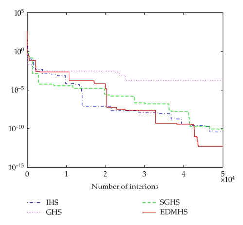
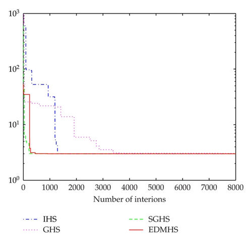
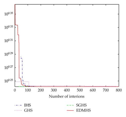
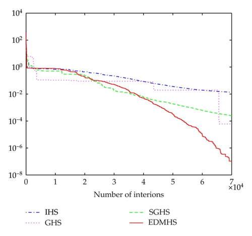
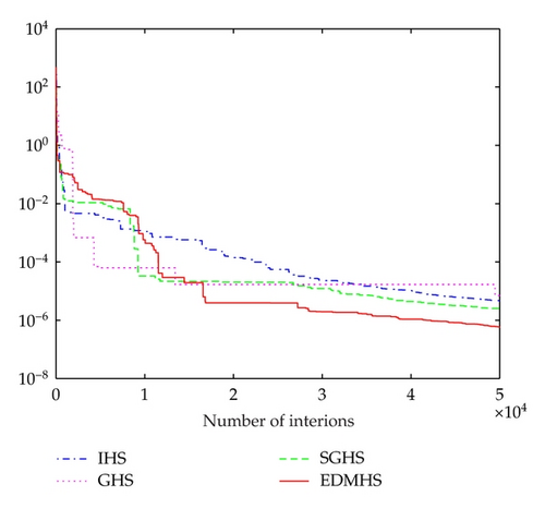
It can be seen from Tables 1–5, comparing with IHS, GHS, and SGHS algorithms, that the EDMHS produces the much better results for four test functions. Figures 1–5 present a typical solution history graph along iterations for the five functions, respectively. It can be observed that four evolution curves of the EDMHS algorithm reach lower level than that of the other compared algorithms. Thus, it can be concluded that overall the EDMHS algorithm outperforms the other methods for the above examples.

Details are in the caption following the image — **Figure 1**
Open in figure viewer PowerPoint

Convergence of Rosenbrock function.

4.2. More Benchmark Problems with 30 Dimensions

To test the performance of the proposed EDMHS algorithm more extensively, we proceed to evaluate and compare the IHS, GHS, SGHS, and EDMHS algorithms based on the following 6 benchmark optimization problems listed in CEC2005 [27] with 30 dimensions.

(1)
Sphere function:
(4.6)
where global optimum x^* = 0 and f(x^*) = 0 for −100 ≤ x_i ≤ 100.
(2)
Schwefel problem:
(4.7)
where global optimum x^* = (420.9687, …, 420.9687) and f(x^*) = −12569.5 for −500 ≤ x_i ≤ 500.
(3)
Griewank function:
(4.8)
where global optimum x^* = 0 and f(x^*) = 0 for −600 ≤ x_i ≤ 600.
(4)
Rastrigin function:
(4.9)
where global optimum x^* = 0 and f(x^*) = 0 for −5.12 ≤ x_i ≤ 5.12.
(5)
Ackley’s function:
(4.10)
where global optimum x^* = 0 and f(x^*) = 0 for −32 ≤ x_i ≤ 32.
(6)
Rosenbrock’s Function:
(4.11)
where global optimum x^* = (1, …, 1) and f(x^*) = 0 for −5 ≤ x_i ≤ 10.

The parameters for the IHS algorithm, HMS = 5, HMCR = 0.9, , bw_min = 0.0001, PAR_min = 0.01, and PAR_max = 0.99 and for the GHS algorithm, HMS = 5, HMCR = 0.9, PAR_min = 0.01, and PAR_max = 0.99.

Table 6 presents the average error (AE) values and standard deviations (SD) over these 30 runs of the compared HS algorithms on the 6 test functions with dimension equal to 30.

Table 6. AE and SD generated by the compared algorithms.

Problem	IHS	IHS	GHS	GHS	SGHS	SGHS	EDMHS	EDMHS
Problem	AE	SD	AE	SD	AE	SD	AE	SD
Sphere	1.27e − 07	1.79e − 07	1.41e − 02	2.36e − 02	5.30e − 07	1.27e − 06	1.07e − 07	1.31e − 07
Schwefel	4.83e − 01	7.06e − 01	2.11e − 02	3.01e − 02	7.70e − 01	1.15e − 00	7.03e − 01	1.61e − 00
Griewank	1.18e − 01	1.87e − 01	8.83e − 02	1.57e − 01	8.02e − 03	1.05e − 02	1.02e − 02	1.51e − 02
Rastrigin	9.72e − 01	1.18e − 00	1.09e − 02	2.05e − 02	1.12e − 00	1.43e − 00	1.48e − 00	1.93e − 00
Ackley	5.11e − 01	6.06e − 01	2.05e − 02	2.83e − 02	2.13e − 01	2.98e − 01	3.34e − 01	3.85e − 01
Rosenbrock	3.37e + 01	4.08e + 01	6.77e + 01	8.97e + 01	3.46e + 01	3.80e + 01	3.17e + 01	4.02e + 01

4.3. Integer Variables Examples

Six commonly used integer programming benchmark problems are chosen to investigate the performance of the EDMHS integer algorithm. For all the examples, the design variables, x_i, i = 1, …, N, are initially structured with random integer values bounded between −100 and 100, respectively. Each problem is run 5 independent replications, each with approximately 800 searches, all the optimal solution vector are obtained.

4.3.1. Test Problem 1

Consider the following:

(4.12)

where x^* = (1,1) ^T and f₁(x^*) = 0, see [14, 21, 28].

4.3.2. Test Problem 2

Consider the following:

(4.13)

where x^* = (0,0, 0,0) ^T and f₂(x^*) = 0, see [14, 21, 28].

4.3.3. Test Problem 3

Consider the following:

(4.14)

where

(4.15)

and f₃(x^*) = 0, see [14, 21, 29].

4.3.4. Test Problem 4

Consider the following:

(4.16)

where x^* = (0,0, 0,0, 0) ^T and f₄(x^*) = 0, see [14, 21, 30].

4.3.5. Test Problem 5

Consider the following:

(4.17)

where x^* = (0,11,22,16,6) ^T and x^* = (10,12,23,17,6) ^T with f₅(x^*) = −737, see [21, 28].

4.3.6. Test Problem 6

Consider the following:

(4.18)

where x^* = (0,1) ^T and f₆(x^*) = −3833.12, see [21, 28].

5. Conclusion

This paper presented an EDMHS algorithm for solving continuous optimization problems and integer optimization problems. The proposed EDMHS algorithm applied a newly designed scheme to generate candidate solution so as to benefit from the good information inherent in the best and the second best solution in the historic HM.

Further work is still needed to investigate the effect of EDMHS and adopt this strategy to solve the real optimization problem.

Acknowlegdments

The research is supported by the Grant from National Natural Science Foundation of China no. 11171373 and the Grant from Natural Science Foundation of Zhejiang Province no. LQ12A01024.

References

1 Geem Z. W., Kim J. H., and Loganathan G. V., A new heuristic optimization algorithm: harmony search, Simulation. (2001) 76, no. 2, 60–68, 2-s2.0-0034974417, https://doi.org/10.1177/003754970107600201.
10.1177/003754970107600201
Web of Science® Google Scholar
2 Geem Z. W. and Choi J. Y., Music composition using harmony search algorithm, Proceedings of the Applications of Evolutionary Computing, April 2007, 593–600, 2-s2.0-34548087100.
Google Scholar
3 Geem Z., Harmony search algorithm for solving sudoku, Knowledge-Based Intelligent Information and Engineering Systems, Springer, 371–378.
Google Scholar
4 Lee K. S. and Geem Z. W., A new structural optimization method based on the harmony search algorithm, Computers and Structures. (2004) 82, no. 9-10, 781–798, 2-s2.0-1842427544, https://doi.org/10.1016/j.compstruc.2004.01.002.
10.1016/j.compstruc.2004.01.002
Web of Science® Google Scholar
5 Saka M. P., Optimum geometry design of geodesic domes using harmony search algorithm, Advances in Structural Engineering. (2007) 10, no. 6, 595–606, 2-s2.0-39449084451, https://doi.org/10.1260/136943307783571445.
10.1260/136943307783571445
Web of Science® Google Scholar
6 Geem Z. and Williams J., Ecological optimization using harmony search, Proceedings of the American Conference on Applied Mathematics, 2008, 24–26.
Google Scholar
7 Ayvaz M. T., Simultaneous determination of aquifer parameters and zone structures with fuzzy c-means clustering and meta-heuristic harmony search algorithm, Advances in Water Resources. (2007) 30, no. 11, 2326–2338, 2-s2.0-34548359352, https://doi.org/10.1016/j.advwatres.2007.05.009.
10.1016/j.advwatres.2007.05.009
Web of Science® Google Scholar
8 Geem Z. W., Harmony search applications in industry, Soft Computing Applications in Industry. (2008) 226, 117–134, 2-s2.0-39449106897, https://doi.org/10.1007/978%2D3%2D540%2D77465%2D5_6.
10.1007/978-3-540-77465-5_6
Google Scholar
9 Geem Z., Music-Inspired Harmony Search Algorithm: Theory and Applications, 2009, 191, Springer.
10.1007/978-3-642-00185-7
Web of Science® Google Scholar
10 Ingram G. and Zhang T., Overview of applications and developments in the harmony search algorithm, Music-Inspired Harmony Search Algorithm. (2009) 191, 15–37, 2-s2.0-62549102999, https://doi.org/10.1007/978%2D3%2D642%2D00185%2D7_2.
10.1007/978-3-642-00185-7_2
Google Scholar
11 Mahdavi M., Fesanghary M., and Damangir E., An improved harmony search algorithm for solving optimization problems, Applied Mathematics and Computation. (2007) 188, no. 2, 1567–1579, https://doi.org/10.1016/j.amc.2006.11.033, 2335651, ZBL1119.65053.
10.1016/j.amc.2006.11.033
Web of Science® Google Scholar
12 Wang C. M. and Huang Y. F., Self-adaptive harmony search algorithm for optimization, Expert Systems with Applications. (2010) 37, no. 4, 2826–2837, 2-s2.0-71349085195, https://doi.org/10.1016/j.eswa.2009.09.008.
10.1016/j.eswa.2009.09.008
Web of Science® Google Scholar
13 Fesanghary M., Mahdavi M., Minary-Jolandan M., and Alizadeh Y., Hybridizing harmony search algorithm with sequential quadratic programming for engineering optimization problems, Computer Methods in Applied Mechanics and Engineering. (2008) 197, no. 33-40, 3080–3091, 2-s2.0-44749086748, https://doi.org/10.1016/j.cma.2008.02.006, ZBL1194.74243.
10.1016/j.cma.2008.02.006
Web of Science® Google Scholar
14 Omran M. G. H. and Mahdavi M., Global-best harmony search, Applied Mathematics and Computation. (2008) 198, no. 2, 643–656, https://doi.org/10.1016/j.amc.2007.09.004, 2405967, ZBL1146.90091.
10.1016/j.amc.2007.09.004
Web of Science® Google Scholar
15 Geem Z. W., Novel derivative of harmony search algorithm for discrete design variables, Applied Mathematics and Computation. (2008) 199, no. 1, 223–230, https://doi.org/10.1016/j.amc.2007.09.049, 2415816, ZBL1146.90501.
10.1016/j.amc.2007.09.049
Web of Science® Google Scholar
16 Pan Q.-K., Suganthan P. N., Tasgetiren M. F., and Liang J. J., A self-adaptive global best harmony search algorithm for continuous optimization problems, Applied Mathematics and Computation. (2010) 216, no. 3, 830–848, https://doi.org/10.1016/j.amc.2010.01.088, 2606991, ZBL1189.65129.
10.1016/j.amc.2010.01.088
Web of Science® Google Scholar
17 Jaberipour M. and Khorram E., Two improved harmony search algorithms for solving engineering optimization problems, Communications in Nonlinear Science and Numerical Simulation. (2010) 15, 3316–3331, https://doi.org/10.1016/j.cnsns.2010.01.009.
10.1016/j.cnsns.2010.01.009
Web of Science® Google Scholar
18 Yadav P., Kumar R., Panda S., and Chang C., An intelligent tuned harmony search algorithm for optimisation, Information Sciences. (2012) 196, 47–72, https://doi.org/10.1016/j.ins.2011.12.035.
10.1016/j.ins.2011.12.035
Web of Science® Google Scholar
19 Pan Q., Suganthan P., Liang J., and Tasgetiren M., A local-best harmony search algorithm with dynamic subpopulations, Engineering Optimization. (2010) 42, 101–117, https://doi.org/10.1080/03052150903104366.
10.1080/03052150903104366
Web of Science® Google Scholar
20 Islam S., Das S., Ghosh S., Roy S., and Suganthan P., An adaptive differential evolution algorithm with novel mutation and crossover strategies for global numerical optimization, IEEE Transactions on Systems, Man, and Cybernetics. (2012) 42, no. 2, 482–500.
10.1109/TSMCB.2011.2167966
PubMed Google Scholar
21 Laskari E., Parsopoulos K., and Vrahatis M., Particle swarm optimization for integer programming, 2, Proceedings of the IEEE Congress on Evolutionary Computation, 1582–1587.
Google Scholar
22 Rosenbrock H. H., An automatic method for finding the greatest or least value of a function, The Computer Journal. (1960) 3, 175–184, 0136042, https://doi.org/10.1093/comjnl/3.3.175.
10.1093/comjnl/3.3.175
Web of Science® Google Scholar
23 Goldstein A. A. and Price J. F., On descent from local minima, Mathematics of Computation. (1971) 25, 569–574, 0312365, https://doi.org/10.1090/S0025%2D5718%2D1971%2D0312365%2DX, ZBL0223.65020.
10.1090/S0025-5718-1971-0312365-X
Web of Science® Google Scholar
24 Eason E. D. and Fenton R. G., A comparison of numerical optimization methods for engineering design, Journal of Engineering for Industry. (1974) 96, no. 1, 196–200, 2-s2.0-0016027933, https://doi.org/10.1115/1.3438296.
10.1115/1.3438296
Google Scholar
25 Colville A., Center I. B. M. C. N. Y. S., and Center I. B. M. C. P .S., A Comparative Study on Nonlinear Programming Codes, 1970, IBM Corporation, Philadelphia Scientific Center.
Web of Science® Google Scholar
26 Conn A., Scheinberg K., and Toint P., On the convergence of derivative-free methods for unconstrained optimization, Approximation Theory and Optimization: Tributes to MJD Powell, 1997, 83–108, 1601691, ZBL1042.90617.
Google Scholar
27 Suganthan P., Hansen N., Liang J., Deb K., Chen Y., Auger A., and Tiwari S., Problem definitions and evaluation criteria for the cec 2005 special session on real-parameter optimization, 2005, no. 2005005, Nanyang Technological University, Singapore.
Google Scholar
28 Glankwahmdee A., Judith S., and Gary L., Unconstrained discrete nonlinear programming, Engineering Optimization. (1979) 4, no. 2, 95–107, 2-s2.0-0018321678, https://doi.org/10.1080/03052157908902410.
10.1080/03052157908902410
Web of Science® Google Scholar
29 Rao S. S. and Rao S. S., Engineering Optimization: Theory and Practice, 2009, John Wiley & Sons, Hoboken, NJ, USA.
Google Scholar
30 Rudolph G., An evolutionary algorithm for integer programming, Proceedings of the 3rd Conference on Parallel Problem Solving from Nature (PPSN ′94), October 1994, Jerusalem, Israel, 139–148.
Google Scholar

Citing Literature

All articles

An Elite Decision Making Harmony Search Algorithm for Optimization Problem

Abstract

1. Introduction