On Kalman Smoothing for Wireless Sensor Networks Systems with Multiplicative Noises
Abstract
The paper deals with Kalman (or H2) smoothing problem for wireless sensor networks (WSNs) with multiplicative noises. Packet loss occurs in the observation equations, and multiplicative noises occur both in the system state equation and the observation equations. The Kalman smoothers which include Kalman fixed-interval smoother, Kalman fixedlag smoother, and Kalman fixed-point smoother are given by solving Riccati equations and Lyapunov equations based on the projection theorem and innovation analysis. An example is also presented to ensure the efficiency of the approach. Furthermore, the proposed three Kalman smoothers are compared.
1. Introduction
The linear estimation problem has been one of the key research topics of control community according to [1]. As is well known, two indexes are used to investigate linear estimation, one is H2 index, and the other is H∞ index. Under the performance of H2 index, Kalman filtering [2–4] is an important approach to study linear estimation besides Wiener filtering. In general, Kalman filtering which usually uses state space equation is better than Wiener filtering, since it is recursive, and it can be used to deal with time-variant system [1, 2, 5]. This has motivated many previous researchers to employ Kalman filtering to study linear time variant or linear time-invariant estimation, and Kalman filtering has been a popular and efficient approach for the normal linear system. However, the standard Kalman filtering cannot be directly used in the estimation on wireless sensor networks (WSNs) since packet loss occurs, and sometimes multiplicative noises also occur [6, 7].
Linear estimation for systems with multiplicative noises under H2 index has been studied well in [8, 9]. Reference [8] considered the state optimal estimation algorithm for singular systems with multiplicative noise, and dynamic noise and noise measurement estimations have been proposed. In [9], we presented the linear filtering for continuous-time systems with time-delayed measurements and multiplicative noises under H2 index.
Wireless sensor networks have been popular these years, and the corresponding estimation problem has attracted many researchers’ attention [10–15]. It should be noted that in the above works, only packet loss occurs. Reference [10] which is an important and ground-breaking reference has considered the problem of Kalman filtering of the WSN with intermittent packet loss, and Kalman filter together with the upper and lower bounds of the error covariance is presented. Reference [11] has developed the work of [10], the measurements are divided into two parts which are sent by different channel under different packet loss rate, and the Kalman filter together with the covariance matrix is given. Reference [14] also develops the result of [11], and the stability of the Kalman filter with Markovian packet loss has been given.
However, the above references mainly focus on the linear systems with packet loss, and they cannot be useful when there are multiplicative noises in the system models [6, 7, 16–18]. For the Kalman filtering problem for wireless sensor networks with multiplicative noises, [16–18] give preliminary results, where [16] has given Kalman filter, [17] deals with the Kalman filter for the wireless sensor networks system with two multiplicative noises and two measurements which are sent by different channels and packet-drop rates, and [18] has given the information fusion Kalman filter for wireless sensor networks with packet loss and multiplicative noises.
In this paper, Kalman smoothing problem including fixed-point smoothing [6], fixed-interval smoothing, and fixed-lag smoothing [7] for WSN with packet loss will be studied. Multiplicative noises both occur in the state equation and observation equation, which will extend the result of works of [8] where multiplicative noises only occur in the state equations. Three Kalman smoothers will be given by recursive equations. The smoother error covariance matrices of fixed-interval smoothing and fixed-lag smoothing are given by Riccati equation without recursion, while the smoother error covariance matrix of fixed-point smoothing is given by recursive Riccati equation and recursive Lyapunov equation, which develops the work of [6, 7], where some main theorems with errors on Kalman smoothing are given.
The rest of the paper is organized as follows. In Section 2, we will present the system model and state the problem to be dealt with in the paper. The main results of Kalman smoother will be given in Section 3. In Section 4, a numerical example will be given to show the result of smoothers. Some conclusion will be drawn in Section 5.
2. Problem Statement
Assumption 2.1. γ(t) (t ≥ 0) is Bernoulli random variable with probability distribution
Assumption 2.2. The initial states x(0), u(t), v(t), and w(t) are all uncorrelated white noises with zero means and known covariance matrices, that is,
The Kalman smoothing problem considered in the paper for the system model (2.1)–(2.3) can be stated in the following three cases.
Problem 1 (fixed-interval smoothing). Given the measurements {y(0), …, y(N)} and scalars {γ(0), …, γ(N)} for a fixed scalar N, find the fixed-interval smoothing estimate of x(t), such that
Problem 2 (fixed-lag smoothing). Given the measurements {y(0), …, y(t)} and scalars {γ(0), …, γ(t)} for a fixed scalar l, find the fixed-lag smoothing estimate of x(t − l), such that
Problem 3 (fixed-point smoothing). Given the measurements {y(0), …, y(N)} and scalars {γ(0), …, γ(N)} for a fixed time instant t, find the fixed-point smoothing estimate of x(t), such that
3. Main Results
In this section, we will give Kalman fixed-interval smoothing, Kalman fixed-lag smoothing, and Kalman fixed-point smoothing for the system model (2.1)–(2.3) and compare them with each other. Before we give the main result, we first give the Kalman filtering for the system model (2.1)–(2.3) which will be useful in the section. We first give the following definition.
Definition 3.1. Given time instants t and j, the estimator is the optimal estimation of ξ(t) given the observation sequences
Remark 3.2. It should be noted that the linear space ℒ{y(0), …, y(t − 1); γ(0), …, γ(t − 1)} means the linear space ℒ{y(0), …, y(t − 1)} under the condition that the scalars γ(0), …, γ(t − 1) are known. So is the linear space ℒ{y(0), …, y(t), y(t + 1), …, y(j); γ(0), …, γ(t), γ(t + 1), …, γ(j)}.
Give the following denotations:
Lemma 3.3.
Proof. Firstly, from (3.2) in Definition 3.1, we have
Next, we show that is an uncorrelated sequence. In fact, for any t, s (t ≠ s), we can assume that t > s without loss of generality, and it follows from (3.7) that
For the convenience of derivation, we will give the orthogonal projection theorem in form of the next theorem without proof, and readers can refer to [4, 5],
Theorem 3.4. Given the measurements {y(0), …, y(t)} and the corresponding innovation sequence in Lemma 3.3, the projection of the state x can be given as
According to a reviewer’s suggestion, we will give the Kalman filter for the system model (2.1)–(2.3) which has been given in [7]
Lemma 3.5. Consider the system model (2.1)–(2.3) with scalars γ(0), …, γ(t + 1) and the initial condition ; the Kalman filter can be given as
Proof. Firstly, according to the projection theorem (Theorem 3.4), we have
Thirdly, by considering (3.7) and Theorem 3.4, we also have
From (2.1) and (3.24), we have
From (2.1), (3.20) can be given directly, and the proof is over.
3.1. Kalman Fixed-Interval Smoother
Theorem 3.7. Consider the system (2.1)–(2.3) with the measurements {y(0), …, y(N)} and scalars {γ(0), …, γ(N)}, Kalman fixed-interval smoother can be given by the following backwards recursive equations:
Proof. From the projection theorem, we have
Noting that x(t) is uncorrelated with w(t + k − 1), u(t + k − 1), and v(t + k − 1) for k = 1, …, N − t, then from (3.5), we have
Next, we will give the proof of covariance matrix P(t∣N). From the projection theorem, we have , and from (3.34), we have
Remark 3.8. The proposed theorem is based on the theorem in [6]. However, the condition of the theorem in [6] is wrong since multiplicative noises w(0), …, w(t) are not known. In addition, the proposed theorem gives the fixed-interval smoother error covariance matrix P(t∣N) which is an important index in Problem 1 and also useful in the comparison with fixed-lag smoother.
3.2. Kalman Fixed-Lag Smoother
Let tl = t − l, and we can give Kalman fixed-lag smoothing estimate for the system model (2.1)–(2.3), which develops [6] in the following theorem.
Theorem 3.9. Consider the system (2.1)–(2.3), given the measurements {y(0), …, y(t)} and scalars {γ(0), …, γ(t)} for a fixed scalar l(l < t), then Kalman fixed-lag smoother can be given by the following recursive equations:
Proof. From the projection theorem, we have
Noting that x(t) is uncorrelated with w(t + k − 1), u(t + k − 1), and v(t + k − 1) for k = 1, …, l, then from (3.5), we have
Next, we will give the proof of covariance matrix P(tl∣t). Since , from (3.41), we have
Remark 3.10. It should be noted that the result of the Kalman smoothing is better than that of Kalman filtering for the normal systems without packet loss since more measurement information is available. However, it is not the case if the measurement is lost, which can be verified in the next section. In addition, in Theorems 3.7 and 3.9, we have changed the predictor type of x(t) or x(tl) in [6] to the filter case of x(t∣t) or x(tl∣tl), which will be more convenient to be compared with Kalman fixed-point smoother (3.45).
3.3. Kalman Fixed-Point Smoother
In this subsection, we will present the Kalman fixed-point smoother by the projection theorem and innovation analysis. We can directly give the theorem which develops [7] as follows.
Theorem 3.11. Consider the system (2.1)–(2.3) with the measurements {y(0), …, y(j)} and scalars {γ(0), …, γ(j)}, then Kalman fixed-point smoother can be given by the following recursive equations:
Proof. The proof of (3.45) and (3.47) can be referred to [7], and we only give the proof of the covariance matrix P(t∣j). From the projection theorem, we have
From (3.50) and considering , then we have
3.4. Comparison
In this subsection, we will give the comparison among the three cases of smoothers. It can be easily seen from (3.31), (3.38), and (3.45) that the smoothers are all given by a Kalman filter and an updated part. To be compared conveniently, the smoother error covariance matrices are given in (3.32), (3.39), and (3.46), which develops the main results in [6, 7] where only Kalman smoothers are given.
It can be easily seen from (3.31) and (3.38) that Kalman fixed-interval smoother is similar to fixed-lag smoother. For (3.31), the computation time is N − t, and it is l in (3.38). For Kalman fixed-interval smoother, the N is fixed, and t is variable, so when t = 0,1, …, N − 1, the corresponding smoother can be given. For Kalman fixed-lag smoother, the l is fixed, and t is variable, so when t = l + 1, l + 2, …, the corresponding smoother can be given. The two smoothers are similar in the form of (3.31) and (3.38). However, it is hard to see which smoother is better from the smoother error covariance matrix (3.32) and (3.39), which will be verified in numerical example.
For Kalman fixed-point smoother in Theorem 3.7, the time t is fixed, and in this case, we can say that Kalman fixed-point smoother is different from fixed-interval and fixed-lag smoother in itself. j can be equal to t + 1, t + 2, ….
4. Numerical Example
In the section, we will give an example to show the efficiency and the comparison of the presented results.
Our aim is to calculate the Kalman fixed-interval smoother of the signal x(t), Kalman fixed-lag smoother of the signal x(tl) for t = l + 1, …, N, and Kalman fixed-point smoother of the signal x(t) for j = t + 1, …, N based on observations , and , respectively. For the Kalman fixed-point smoother , we can set t = 30.
According to Theorem 3.7, the computation of the Kalman fixed-interval smoother can be summarized in three steps as shown below.
Step 1. Compute Π(t + 1), P(t + 1), , and by (3.20), (3.19), (3.18), and (3.17) in Lemma 3.5 for t = 0, …, N − 1, respectively.
Step 2. t ∈ [0, N] is set invariant compute P(t, k) by (3.33) for k = 1, …, N − t; with the above initial values P(t, 0) = P(t).
Step 3. Compute the Kalman fixed-interval smoother by (3.31) for t = 0, …, N with fixed N.
Similarly, according to Theorem 3.9, the computation of the Kalman fixed-lag smoother can be summarized in three steps as shown below.
Step 1. Compute Π(tl + k + 1), P(tl + k + 1), , and by (3.20), (3.19), (3.18), and (3.17) in Lemma 3.5 for t > l and k = 1, …, l, respectively.
Step 2. t ∈ [0, N] is set invariant; compute P(tl, k) by (3.40) for k = 1, …, l with the above initial values P(tl, 0) = P(tl).
Step 3. Compute the Kalman fixed-lag smoother by (3.38) for t > l.
According to Theorem 3.11, the computation of Kalman fixed-point smoother can be summarized in three steps as shown below.
Step 1. Compute Π(t + 1), P(t + 1), , and by (3.20), (3.19), (3.18) and (3.17) in Lemma 3.5 for t = 0, …, N − 1, respectively.
Step 2. Compute P(t, k) by (3.47) for k = 1, …, j − t with the initial value P(t, 0) = P(t).
Step 3. Compute the Kalman fixed-point smoother by (3.45) for j = t + 1, …, N.
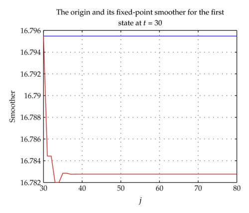
The tracking performance of Kalman fixed-point smoother is drawn in Figures 1 and 2, and the line is based on the fixed time t = 30, and the variable is j. It can be easily seen from the above two figures that the smoother is changed much at first, and after the time j = 35, the fixed-point smoother is fixed, that is, the smoother at time t = 30 will take little effect on y(j), y(j + 1), … due to packet loss. In addition, at time j = 30, the estimation (filter) is more closer to the origin than other j > 30, which shows that Kalman filter is better than fixed-point smoother for WSN with packet loss. In fact, the smoothers below are also not good as filter.
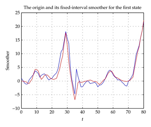
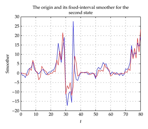
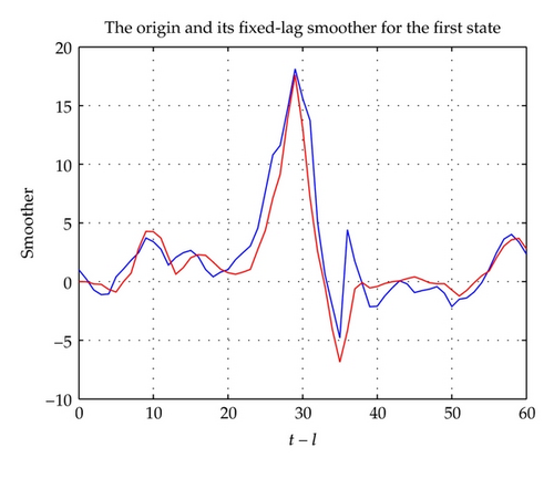
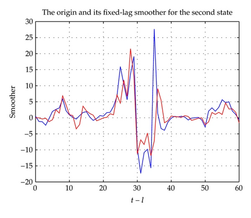
The fixed-interval smoother is given in Figures 3 and 4, and the tracking performance of the fixed-lag smoother is given in Figures 5 and 6. From the above figures, they can estimate the origin signal in general.
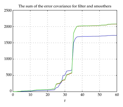
In addition, according to the comparison part in the end of last section, we give the comparison of the sum of the error covariance of the fixed-interval and fixed-lag smoother (the fixed-point smoother is different from the above two smoother, so its error covariance is not necessary to be compared with, which has been explained at the end of last section), and we also give the sum of the error covariance of Kalman filter, and they are all drawn in Figure 7. As seen from Figure 7, it is hard to say which smoother is better due to packet loss, and the result of smoothers is not better than filter.

5. Conclusion
In this paper, we have studied Kalman fixed-interval smoothing, fixed-lag smoothing [6], and fixed-point smoothing [7] for wireless sensor network systems with packet loss and multiplicative noises. The smoothers are given by recursive equations. The smoother error covariance matrices of fixed-interval smoothing, and fixed-lag smoothing are given by Riccati equation without recursion, while the smoother error covariance matrix of fixed-point smoothing is given by recursive Riccati equation and recursive Lyapunov equation. The comparison among the fixed-point smoother, fixed-interval smoother and fixed-lag smoother has been given, and numerical example verified the proposed approach. The proposed approach will be useful to study more difficult problems, for example, the WSN with random delay and packet loss [19].
Disclosure
X. Lu is affiliated with Shandong University of Science and Technology and also with Shandong University, Qingdao, China. H. Wang and X. Wang are affiliated with Shandong University of Science and Technology, Qingdao, China.
Acknowledgment
This work is supported by National Nature Science Foundation (60804034), the Scientific Research Foundation for the Excellent Middle-Aged and Youth Scientists of Shandong Province (BS2012DX031), the Nature Science Foundation of Shandong Province (ZR2009GQ006), SDUST Research Fund (2010KYJQ105), the Project of Shandong Province Higher Educational Science, Technology Program (J11LG53) and “Taishan Scholarship” Construction Engineering.


