Application of the Variational Iteration Method to Strongly Nonlinear q-Difference Equations
Abstract
The theory of approximate solution lacks development in the area of nonlinear q-difference equations. One of the difficulties in developing a theory of series solutions for the homogeneous equations on time scales is that formulas for multiplication of two q-polynomials are not easily found. In this paper, the formula for the multiplication of two q-polynomials is presented. By applying the obtained results, we extend the use of the variational iteration method to nonlinear q-difference equations. The numerical results reveal that the proposed method is very effective and can be applied to other nonlinear q-difference equations.
1. Introduction
A time scale is a nonempty closed subset of real numbers. Recently, much research activity has focused on the theory and application of the q-calculus. For example, the q-calculus has being given a financial meaning by Muttel [1] and is applied to pricing the financial derivatives. Many real world problems are now formulated as q-difference equations. Nonlinear q-difference equations, as well as their analytic and numerical solutions, play an important role in various fields of science and engineering, especially in nonlinear physical science, since their solutions can provide more inside into the physical aspects of the problems.
Solutions of linear differential equations on time scales have been studies and published during the past two decades. One area lacking in development is the theory of approximate solutions on nonlinear q-difference equations. Recent developments in the theory of approximate solution have aroused further interest in the discussion of nonlinear q-difference equations.
One of the difficulties in developing a theory of series solutions for linear or nonlinear homogeneous equations on time scales is that formulas for multiplication of two generalized polynomials are not easily found. Haile and Hall [2] provided an exact formula for the multiplication of two generalized polynomials if the time scale had constant graininess. Using the obtained results, the series solutions for linear dynamic equations were proposed on the time scales ℝ and 𝕋 = hℤ (difference equations with step size h). For generalized time scales, Mozyrska and Pawtuszewicz [3] presented the formula for the multiplication of the generalized polynomials of degree one and degree n ∈ ℕ.
The variational iteration method proposed by He [4] has been proved by many authors to be a powerful mathematical tool for analysing the nonlinear problems on ℝ (the set of real numbers). The advantages of this method include (i) that it can be applied directly to all types of difference equations, and (ii) that it reduces the size of computational work while maintaining the high accuracy of the numerical solution. For the nonlinear q-difference equations, the approximate solution obtained by using the variational iteration method may not yet been found.
This paper is organized as follows: in Section 2 basic ideas on q-calculus are introduced; in Section 3, the multiplication of two q-polynomials is demonstrated; in Section 4, the variational iteration method is applied to find an approximate solution of strongly nonlinear damped q-difference equations; in Section 5, the numerical results and the approximate solutions, which were very close, are presented; finally, a concise conclusion is provided in Section 6.
2. Introduction to q-Calculus
Definition 2.1. Assume that is a function and . The q-derivative [6] at t is defined by
A q-difference equation is an equation that contains q-derivatives of a function defined on .
Definition 2.2. On the time scale , the q-polynomials are defined recursively as follows:
Using q-polynomials, Agarwal and Bohner [7] gave a Taylor’s formula for functions on a general time scale. On Taylor’s formula is written follows.
Theorem 2.3. Let n ∈ ℕ. Suppose that f is n times differentiable on . Let . Then one has
3. Multiplication of Two q-Polynomials
The purpose of this section is to propose a production rule of two q-polynomials at 0 [8] which will be used to derive an approximate solution in the following section.
Theorem 3.1. Let hi(t, 0) and hj(t, 0) be two q-polynomials at zero. One has
Proof. Since
Proposition 3.2. Let hi(t, 0) and hj(t, 0) be any two q-polynomials. We have
4. Variational Iteration Method
4.1. Basic Ideas of Variational Iteration Method
4.2. Approximate Solution to Nonlinear Damped q-Equations
5. Numerical Method
6. Numerical Results
The theoretical considerations introduced in previous sections are illustrated with examples, where the approximate solutions are compared with the numerical solutions.
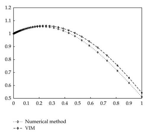
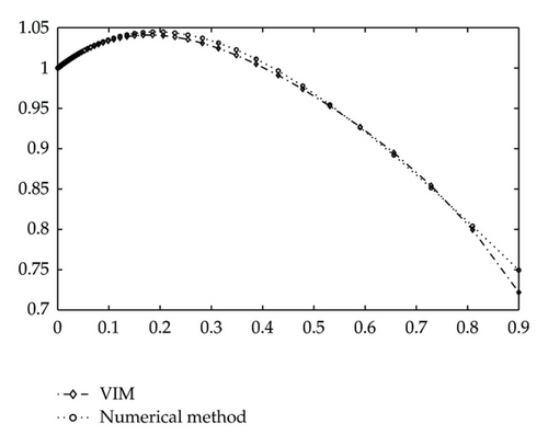
Example 6.1. Consider the underdamped cases with (i) 2γ = 0.1, γ1 = 0.1, ε = 1, and Ω = 1; and (ii) 2γ = 0.1, γ1 = 2.5, ε = 1 and Ω = 1. As the initial conditions are given as x(0) = 1 and xΔ(0) = 0.5, we begin with the initial approximation x0 = 1 + 0.5t. By the variational iteration formula (4.11), we obtain the first few components of xn(t). In the same manner the rest of the components of the iteration formula are obtained using the symbolic toolbox in the Matlab package.
For Case (i) The first two components of xn are obtained as
For case (ii) The first two components of xn are obtained as
The responses of x(t) are shown in Figures 1 and 2 for cases (i) and (ii), respectively.
Example 6.2. In this example, we consider the overdamped cases with (iii) 2γ = 2.5, γ1 = 0.1, ε = 1, and Ω = 1; and (iv) 2γ = 2.5, γ1 = 2.5, ε = 1, and Ω = 1. As the initial conditions are given as x(0) = 1 and xΔ(0) = 0.5, we begin with the initial approximation x0 = 1 + 0.5t. By the variational iteration formula (4.11), we obtain the first few components of xn(t). In the same manner the rest of the components of the iteration formula were obtained using the symbolic toolbox in the Matlab package.
For Case (iii) The first two components of xn are obtained as
For Case (iv) The first two components of xn are obtained as
The responses of x(t) are shown in Figures 3 and 4 for cases (iii) and (iv), respectively.
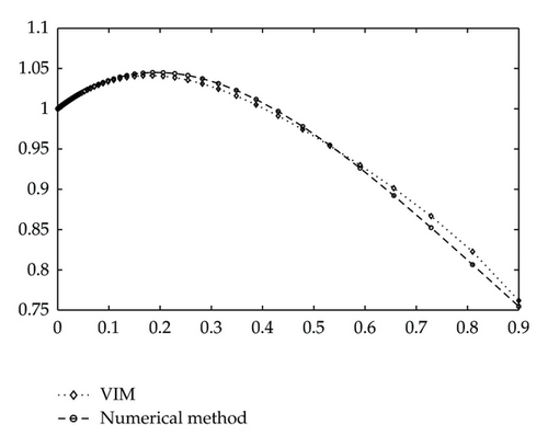
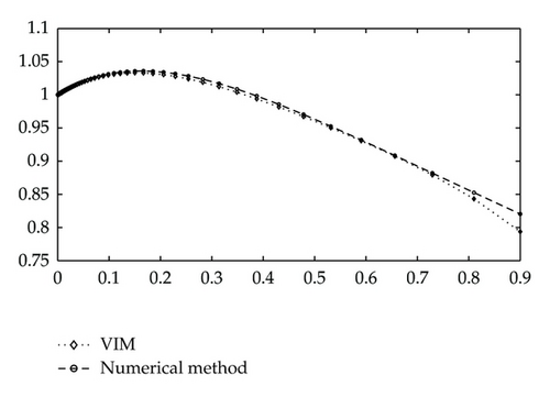
These figures and the maximum/average errors indicate that the approximate solution is close to the numerical results.
7. Conclusion
In the area of q-calculus, the formula for the multiplication of two q-polynomials has long been in need of development. In this paper, we have presented the aforementioned formula, overcoming the previous difficulties in developing a theory of series solutions for the nonlinear q-difference equations. The goal of this paper was to extend the use of the variational iteration method to strongly nonlinear damped q-difference equations. The numerical results have demonstrated that the approximate solution obtained by the variational iteration method is very accurate. Therefore, the proposed method is very effective and can be applied to other nonlinear q-equations.


