This paper studies the second moment stability of a discrete-time jump linear system with real states and the system matrix switching in a Markovian fashion. A sufficient stability condition was proposed by Fang and Loparo (2002), which only needs to check the eigenvalues of a deterministic matrix and is much more computationally efficient than other equivalent conditions. The proof to the necessity of that condition, however, is a challenging problem. In the paper by Costa and Fragoso (2004), a proof was given by extending the state domain to the complex space. This paper proposes an alternative necessity proof, which does not need to extend the state domain. The proof in this paper demonstrates well the essential properties of the Markov jump systems and achieves the desired result in the real state space.

1. Introduction

1.1. Background of the Discrete-Time Markov Jump Linear Systems

This paper studies the stability condition of discrete-time jump linear systems in the real state domain. In a jump linear system, the system parameters are subject to abrupt jumps. We are concerned with the stability condition when these jumps are governed by a finite Markov chain. A general model is shown as follows:

()

where x[k] ∈ Rⁿ is the state and {q[k]} is a discrete-time Markov chain with a finite state space {q₁, q₂, …, q_N} and a transition matrix

, where q_ij = P(q[k + 1] = q_j∣q[k] = q_i). x₀ ∈ Rⁿ is the initial state. q₀ is the initial Markov state, whose distribution is denoted as p = [p₁ p₂ ⋯ p_N] with p_i = P(q₀ = q_i). {q[k]} is assumed to be a time-homogeneous aperiodic Markov chain. When q[k] = q_i, A[q[k]] = A_i(i = 1, …, N), that is, A[q[k]] switches among

. A compound matrix is constructed from A_i as

()

where

denotes an identity matrix with the order of n² and ⊗ denotes the Kronecker product [1]. A brief introduction on the Kronecker product will be given in Section 2.1.

For the jump linear system in (1.1), the first question to be asked is “is the system stable?” There has been plenty of work on this topic, especially in 90s, [2–6]. Recently this topic has caught academic interest again because of the emergence of networked control systems [7]. Networked control systems often suffer from the network delay and dropouts, which may be modelled as Markov chains, so that networked control systems can be classified into discrete-time jump linear systems [8–11]. Therefore, the stability of the networked control systems can be determined through studying the stability of the corresponding jump linear systems. Before proceeding further, we review the related work.

1.2. Related Work

At the beginning, the definitions of stability of jump linear systems are considered. In [6], three types of second moment stability are defined.

Definition 1.1. For the jump linear system in (1.1), the equilibrium point 0 is

(1)
stochastically stable, if, for every initial condition (x[0] = x₀, q[0] = q₀),
()
where ∥·∥ denotes the 2-norm of a vector;
(2)
mean square stable (MSS), if, for every initial condition (x₀, q₀),
()
(3)
exponentially mean square stable, if, for every initial condition (x₀, q₀), there exist constants 0 < α < 1 and β > 0 such that for all k ≥ 0,
()
where α and β are independent of x₀ and q₀.

In [6], the above 3 types of stabilities are proven to be equivalent. So we can study mean square stability without loss of generality. In [6], a necessary and sufficient stability condition is proposed.

Theorem 1.2 (see [6].)The jump linear system in (1.1) is mean square stable, if and only if, for any given set of positive definite matrices {W_i : i = 1, …, N}, the following coupled matrix equations have unique positive definite solutions {M_i : i = 1, …, N}:

()

Although the above condition is necessary and sufficient, it is difficult to verify because it claims validity for any group of positive definite matrices {W_i : i = 1, …, N}. A more computationally efficient testing criterion was, therefore, pursued [3, 4, 12–15]. Theorem 1.3 gives a sufficient mean square stability condition.

Theorem 1.3 (see [4], [12].)The jump linear system in (1.1) is mean square stable, if all eigenvalues of the compound matrix A_[2] in (1.2) lie within the unit circle.

Remark 1.4. By Theorem 1.3, the mean square stability of a jump linear system can be reduced to the stability of a deterministic system in the form y_k+1 = A_[2]y_k [13]. Thus the complexity of the stability problem is greatly reduced. Theorem 1.3 only provides a sufficient condition for stability. The condition was conjectured to be necessary as well [2, 15]. In the following, we briefly review the research results related to Theorem 1.3.

In [14], Theorem 1.3 was proven to be necessary and sufficient for a scalar case, that is, A_i(i = 1, …, N) are scalar. In [15], the necessity of Theorem 1.3 was proven for a special case with N = 2 and n = 2. In [4, 12], Theorem 1.3 was asserted to be necessary and sufficient for more general jump linear systems. Specifically, Bhaurucha [12] considered a random sampling system with the sampling intervals governed by a Markov chain while Mariton [4] studied a continuous-time jump linear system. Although their sufficiency proof is convincing, their necessity proof is incomplete.

The work in [3] may shed light on the proof of the necessity of Theorem 1.3. In [3], a jump linear system model being a little different from (1.1) is considered. The difference lies in

(i)
x[k] ∈ Cⁿ, where C stands for the set of complex numbers,
(ii)
x₀ ∈ S_c, where S_c is the set of complex vectors with finite second-order moments in the complex state space.

The mean square stability in [3] is defined as

()

where * stands for the conjugate transpose. Corresponding to the definition in (1.7), the mean square stability in (1.4) can be eewritten into (because x[k] ∈ Rⁿ in (1.4), there is no difference between x^T[k] and x^*[k]),

()

where S_j is the set of all vectors in Rⁿ. For any vector x ∈ Rⁿ, we can treat it as a random vector with a single element in Rⁿ, and also a random vector in Cⁿ. Of course, such random vectors have finite second-order moments. Therefore, we know

()

It can be seen that the mean square stability in (1.7) requires stronger condition (x₀ ∈ S_c) than the one in (1.8) (x₀ ∈ S_j). When A_i(i = 1, …, N) are real matrices, a necessary and sufficient stability condition was given in the complex state domain.

Theorem 1.5 (see [3].)The jump linear system in (1.1) (with complex states) is mean square stable in the sense of (1.7) if and only if A_[2] is Schur stable.

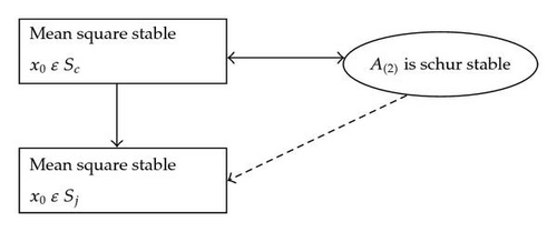
Due to the relationship of S_j ⊂ S_c and Theorem 1.5, we can establish the relationship diagram in Figure 1. As it shows, the Schur stability of A_[2] is a sufficient condition for mean square stability with x₀ ∈ S_j at the first look.

Details are in the caption following the image — **Figure 1**
Open in figure viewer PowerPoint

Relationship between different senses of mean square stability.

We are still wondering “whether the condition in Theorem 1.3 is necessary too?” the answer is definitely “yes.” That necessity was conjectured in [2]. A proof to the necessity of that condition was first given in [16], which extends the state domain to the complex space and establishes the desired necessity in the stability sense of (1.7). As mentioned before, our concerned stability (in the sense of (1.8)) is weaker than that in (1.7). This paper proves that the weaker condition in (1.8) still yields the schur stability of A_[2], that is, the necessity of theorem 1.3 is confirmed. This paper confines the state to the real space domain and makes the best use of the essential properties of the markov jump linear systems to reach the desired necessity goal. In Section 2, a necessary and sufficient version of Theorem 1.3 is stated and its necessity is strictly proven. In Section 3, final remarks are placed.

2. A Necessary and Sufficient Condition for Mean Square Stability

This section will give a necessary and sufficient version of Theorem 1.3. Throughout this section, we will define mean square stability in the sense of (1.4) (x₀ ∈ S_j). At the beginning, we will give a brief introduction to the Kronecker product and list some of its properties. After then, the main result, a necessary and sufficient condition for the mean square stability, is presented in Theorem 2.1 and its necessity is proven by direct matrix computations.

2.1. Mathematical Preliminaries

Some of the technical proofs in this paper make use of the Kronecker product, ⊗ [1]. The Kronecker product of two matrices A = (a_ij) _M×N, B = (b_pq) _P×Q is defined as

()

For simplicity, A ⊗ A is denoted as A^[2] and A ⊗ A^[n] is denoted as A^[n+1](n ≥ 2).

For two vectors x and y, x ⊗ y simply rearranges the columns of xy^T into a vector. So for two stochastic processes {x[n]} and {y[n]}, lim _n→∞E[x[n] ⊗ y[n]] = 0 if and only if lim _n→∞E[x[n]y^T[n]] = 0. Furthermore, if lim _n→∞E[x^[2][n]] = 0 and lim _n→∞E[y^[2][n]] = 0, then

()

The following property of the Kronecker product will be frequently used in the technical proofs

()

where A_i, B_i(i = 1,2, …, n) are all matrices with appropriate dimensions.

Our computations need two linear operators, vec and devec. The vec operator transforms a matrix A = (a_ij) _M×N into a vector as

()

The devec operator inverts the vec operator for a square matrix, that is,

()

where A is a square matrix.

2.2. Main Results

Theorem 2.1. The jump linear system in (1.1) is mean square stable if and only if A_[2] is Schur stable, that is, all eigenvalues of A_[2] lie within the unit circle.

There are already some complete proofs for sufficiency of Theorem 2.1, [3, 12, 13]. So we will focus on the necessity proof. Throughout this section, the following notational conventions will be followed.

The initial condition of the jump linear system in (1.1) is denoted as x[0] = x₀, q[0] = q₀ and the distribution of q₀ is denoted as p = [p₁ p₂ ⋯ p_N] (P(q[0] = q_i∣q₀) = p_i).

The system transition matrix in (1.1) is defined as

()

where I_n is an identity matrix with the order of n. With this matrix, the system’s state at time instant k can be expressed as

()

A conditional expectation is defined as

()

where i = 1,2, …, N. Specially

(i = 1, …, N). Based on the definition of Φ_i[k], we obtain

()

By combining all Φ_i[k](i = 1,2, …, N) into a bigger matrix, we define

()

Thus,

The necessity proof of Theorem 2.1 needs the following three preliminary Lemmas.

Lemma 2.2. If the jump linear system in (1.1) is mean square stable, then

()

Proof of Lemma 2.2. Because the system is mean square stable, we get

()

The expression of x[k] = Φ(k; 0)x₀ yields

()

Φ(k; 0) is an n × n matrix. So we can denote it as Φ(k; 0) = [a₁(k), a₂(k), …, a_n(k)], where a_i(k) is a column vector. By choosing x₀ = e_i (e_i is an R^n×1 vector with the ith element as 1 and the others as 0), (2.13) yields

()

By the definition of the Kronecker product, we know

()

So (2.14) yields

()

Lemma 2.3. If the jump linear system in (1.1) is mean square stable, then

()

Proof of Lemma 2.3. Choose any z₀, w₀ ∈ Rⁿ. Lemma 2.2 guarantees

()

By the definition of the Kronecker product, we know

()

By (2.8), (2.9), and (2.19), we get

()

Because P(q[k] = q_i | q₀) ≥ 0 and

, the combination of (2.18) and (2.20) yields

()

Φ(k; 0) is an n × n matrix. So it can be denoted as Φ(k; 0) = (a_mj(k)) _{m=1,…,n;j=1,…,n}. In (2.21), we choose z₀ = e_m and w₀ = e_j and get

()

where i = 1,2, …, N, m = 1, …, n and j = 1, …, n. By the definition of Φ_i[k], we know the elements of Φ_i[k] take the form of

()

where m₁, m₂, j₁, j₂ = 1, …, n. So (2.22) guarantees

()

Lemma 2.4. V_Φ[k] is governed by the following dynamic equation

()

with

Proof of Lemma 2.4. By the definition in (2.8), we can recursively compute Φ_i[k] as follows:

()

Because Φ(k − 1; 0) depends on only {q[k − 2], q[k − 3], …, q[0]} and the jump sequence {q[k]} is Markovian, we know

()

P(q[k] = q_i∣q₀)P(q[k − 1] = q_j∣q[k] = q_i, q₀) can be computed as

()

Substituting (2.27) and (2.28) into the expression of Φ_i[k], we get

()

After combining Φ_i[k](i = 1,2, …, N) into V_Φ[k] as (2.10), we get

()

We can trivially get V_Φ[0] from Φ_i[0] by (2.10).

Proof of Necessity of Theorem 2.1. By Lemma 2.3, we get

()

By Lemma 2.4, we get

and

. Therefore, (2.31) yields

()

for any p (the initial distribution of q₀).

is an Nn² × Nn² matrix. We can write as where Aⁱ(n)(i = 1, …, N) is an Nn² × n² matrix. By taking p_i = 1 and p_j = 0(j = 1, …, i − 1, i + 1, …, N), (2.32) yields

()

Thus we can get

()

So A_[2] is Schur stable. The proof is completed.

3. Conclusion

This paper presents a necessary and sufficient condition for the second moment stability of a discrete-time Markovian jump linear system. Specifically this paper provides proof for the necessity part. Different from the previous necessity proof, this paper confines the state domain to the real space. It investigates the structures of relevant matrices and make a good use of the essential properties of Markov jump linear systems, which may guide the future research on such systems.

Acknowledgment

This work was supported in part by the National Natural Science Foundation of China (60904012), the Program for New Century Excellent Talents in University (NCET-10-0917) and the Doctoral Fund of Ministry of Education of China (20093402120017).

References

1 Bellman R., Introduction to Matrix Analysis, 1960, McGraw-Hill, New York, NY, USA, 0122820.
Google Scholar
2 Fang Y. and Loparo K. A., Stochastic stability of jump linear systems, IEEE Transactions on Automatic Control. (2002) 47, no. 7, 1204–1208, https://doi.org/10.1109/TAC.2002.800674, 1911501.
10.1109/TAC.2002.800674
Web of Science® Google Scholar
3 Costa O. L. V. and Fragoso M. D., Stability results for discrete-time linear systems with Markovian jumping parameters, Journal of Mathematical Analysis and Applications. (1993) 179, no. 1, 154–178, https://doi.org/10.1006/jmaa.1993.1341, 1244955, ZBL0790.93108.
10.1006/jmaa.1993.1341
Web of Science® Google Scholar
4 Mariton M., Jump Linear Systems in Automatic Control, 1990, Marcel Dekker.
Web of Science® Google Scholar
5 Feng X., Loparo K. A., Ji Y., and Chizeck H. J., Stochastic stability properties of jump linear systems, IEEE Transactions on Automatic Control. (1992) 37, no. 1, 38–53, https://doi.org/10.1109/9.109637, 1139614, ZBL0747.93079.
10.1109/9.109637
Web of Science® Google Scholar
6 Ji Y., Chizeck H. J., Feng X., and Loparo K. A., Stability and control of discrete-time jump linear systems, Control Theory and Advanced Technology. (1991) 7, no. 2, 247–270, 1117531.
Web of Science® Google Scholar
7 Beldiman O., Walsh G. C., and Bushnell L., Predictors for networked control systems, American Control Conference, June 2000, 2347–2351, 2-s2.0-0034542676.
Google Scholar
8 Nilsson J., Real-time control systems with delays, Ph.D. dissertation, 1998, Lund Institute of Technology.
Google Scholar
9 Zhang W., Branicky M. S., and Phillips S. M., Stability of networked control systems, IEEE Control Systems Magazine. (2001) 21, no. 1, 84–97, 2-s2.0-0034831393, https://doi.org/10.1109/37.898794.
10.1109/37.898794
CAS Web of Science® Google Scholar
10 Seiler P. and Sengupta R., Analysis of communication losses in vehicle control problems, American Control Conference, June 2001, 1491–1496, 2-s2.0-0034857808.
Google Scholar
11 Lincoln B. and Cervin A., Jitterbug: a tool for analysis of real-time control performance, IEEE Conference on Decision and Control, December 2002, 1319–1324, 2-s2.0-0036990396.
Google Scholar
12 Bhaurucha B., On the stability of randomly varying systems, Ph.D. dissertation, 1961, University of California, Berkeley, Calif, USA.
Google Scholar
13 Fang Y., Stability analysis of linear control systems with uncertain parameters, Ph.D. dissertation, 1994, Case Western Reserve University.
Google Scholar
14 Gray W. S., Gonzàlez O. R., and Patilkulkarni S., Stability of digital control systems subject to jump linear random perturbations, IEEE Confernce on Decision and Control, December 2000, 1154–1159, 2-s2.0-0034439216.
Google Scholar
15 Dong X., Stochastic stability of discrete-time jump linear systems, Chinese Control Conference, 2003.
Google Scholar
16 Costa O. L. V. and Fragoso M. D., Comments on: ‘Stochastic stability of jump linear systems’, IEEE Transactions on Automatic Control. (2004) 49, no. 8, 1414–1416, https://doi.org/10.1109/TAC.2004.832654, 2078259.
10.1109/TAC.2004.832654
Web of Science® Google Scholar

Citing Literature

All articles

A New Proof to the Necessity of a Second Moment Stability Condition of Discrete-Time Markov Jump Linear Systems with Real States

Abstract

1. Introduction

1.1. Background of the Discrete-Time Markov Jump Linear Systems

1.2. Related Work

2. A Necessary and Sufficient Condition for Mean Square Stability

2.1. Mathematical Preliminaries

2.2. Main Results

3. Conclusion

Acknowledgment

References

Citing Literature

Figures

References

Information

About Wiley Online Library

Help & Support

Opportunities

Connect with Wiley