Volume 2012, Issue 1 626717

Research Article

Open Access

An Improved Particle Swarm Optimization for Solving Bilevel Multiobjective Programming Problem

Corresponding Author

Tao Zhang

[email protected]

State Key Laboratory of Water Resources and Hydropower Engineering Science, Wuhan University, Wuhan 430072, China whu.edu.cn

School of Information and Mathematics, Yangtze University, Jingzhou 434023, China yangtzeu.edu.cn

Search for more papers by this author

Tiesong Hu,

Tiesong Hu

State Key Laboratory of Water Resources and Hydropower Engineering Science, Wuhan University, Wuhan 430072, China whu.edu.cn

Search for more papers by this author

Yue Zheng,

Yue Zheng

College of Mathematics and Computer Sciences, Huanggang Normal University, Huanggang 438000, China

Search for more papers by this author

Xuning Guo,

Xuning Guo

State Key Laboratory of Water Resources and Hydropower Engineering Science, Wuhan University, Wuhan 430072, China whu.edu.cn

Search for more papers by this author

Tao Zhang,

Corresponding Author

Tao Zhang

[email protected]

State Key Laboratory of Water Resources and Hydropower Engineering Science, Wuhan University, Wuhan 430072, China whu.edu.cn

School of Information and Mathematics, Yangtze University, Jingzhou 434023, China yangtzeu.edu.cn

Search for more papers by this author

Tiesong Hu,

Tiesong Hu

State Key Laboratory of Water Resources and Hydropower Engineering Science, Wuhan University, Wuhan 430072, China whu.edu.cn

Search for more papers by this author

Yue Zheng,

Yue Zheng

College of Mathematics and Computer Sciences, Huanggang Normal University, Huanggang 438000, China

Search for more papers by this author

Xuning Guo,

Xuning Guo

State Key Laboratory of Water Resources and Hydropower Engineering Science, Wuhan University, Wuhan 430072, China whu.edu.cn

Search for more papers by this author

First published: 10 April 2012

https://doi.org/10.1155/2012/626717

Citations: 21

Academic Editor: Debasish Roy

Share a link

Email
Wechat
Bluesky

Abstract

An improved particle swarm optimization (PSO) algorithm is proposed for solving bilevel multiobjective programming problem (BLMPP). For such problems, the proposed algorithm directly simulates the decision process of bilevel programming, which is different from most traditional algorithms designed for specific versions or based on specific assumptions. The BLMPP is transformed to solve multiobjective optimization problems in the upper level and the lower level interactively by an improved PSO. And a set of approximate Pareto optimal solutions for BLMPP is obtained using the elite strategy. This interactive procedure is repeated until the accurate Pareto optimal solutions of the original problem are found. Finally, some numerical examples are given to illustrate the feasibility of the proposed algorithm.

1. Introduction

Bilevel programming problem (BLPP) arises in a wide variety of scientific and engineering applications including optimal control, process optimization, game-playing strategy development, and transportation problem Thus, the BLPP has been developed and researched by many scholars. The reviews, monographs, and surveys on the BLPP can refer to [1–11]. Moreover, the evolutionary algorithms (EA) have been employed to address BLPP in papers [12–16].

However, the bilevel multiobjective programming problem (BLMPP) has seldom been studied. Shi and Xia [17, 18], Abo-Sinna and Baky [19], Nishizaki and Sakawa [20], and Zheng et al. [21] presented an interactive algorithm for BLMPP. Eichfelder [22] presented a method for solving nonlinear bilevel multiobjective optimization problems with coupled upper level constraints. Thereafter, Eichfelder [23] developed a numerical method for solving nonlinear nonconvex bilevel multiobjective optimization problems. In recent years, the metaheuristic has attracted considerable attention as an alternative method for BLMPP. For example, Deb and Sinha [24–26] as well as Sinha and Deb [27] discussed BLMPP based on evolutionary multiobjective optimization principles. Based on those studies, Deb and Sinha [28] proposed a viable and hybrid evolutionary-local-search-based algorithm and presented challenging test problems. Sinha [29] presented a progressively interactive evolutionary multiobjective optimization method for BLMPP.

Particle swarm optimization (PSO) is a relatively novel heuristic algorithm inspired by the choreography of a bird flock, which has been found to be quite successful in a wide variety of optimization tasks [30]. Due to its high speed of convergence and relative simplicity, the PSO algorithm has been employed by many researchers for solving BLPPs. For example, Li et al. [31] proposed a hierarchical PSO for solving BLPP. Kuo and Huang [32] applied the PSO algorithm for solving bilevel linear programming problem. Gao et al. [33] presented a method to solve bilevel pricing problems in supply chains using PSO. However, it is worth noting that the papers mentioned above are only for bilevel single objective problems.

In this paper, an improved PSO is presented for solving BLMPP. The algorithm can be outlined as follows. The BLMPP is transformed to solve multiobjective optimization problems in the upper level and the lower level interactively by an improved PSO. And a set of approximate Pareto optimal solutions for BLMPP is obtained using the elite strategy. The above interactive procedure is repeated for a predefined count, and then the accurate Pareto optimal solutions of the BLMPP will be achieved. Towards these ends, the rest of the paper is organized as follows. In Section 2, the problem formulation is provided. The proposed algorithm for solving bilevel multiobjective problem is presented in Section 3. In Section 4, some numerical examples are given to demonstrate the proposed algorithm, while the conclusion is reached in Section 5.

2. Problem Formulation

Let

, and

. The general model of the BLMPP can be written as follows:

()

where F(x, y) and f(x, y) are the upper level and the lower level objective functions, respectively. G(x, y) and g(x, y) denote the upper level and the lower level constraints, respectively. Let S = {(x, y)G(x, y) ≥ 0, g(x, y) ≥ 0}, X = {x∣∃ y, G(x, y) ≥ 0, g(x, y) ≥ 0}, S(x) = {y∣g(x, y) ≥ 0}, and for the fixed x ∈ X, let

denote the weak efficiency set of solutions to the lower level problem, the feasible solution set of problem (2.1) is denoted as

Definition 2.1. For a fixed x ∈ X, if y is a Pareto optimal solution to the lower level problem, then (x, y) is a feasible solution to the problem (2.1).

Definition 2.2. If (x^*, y^*) is a feasible solution to the problem (2.1) and there are no (x, y) ∈ IR, such that F(x, y)≺F(x^*, y^*), then (x^*, y^*) is a Pareto optimal solution to the problem (2.1), where “≺” denotes Pareto preference.

For problem (2.1), it is noted that a solution (x^*, y^*) is feasible for the upper level problem if and only if y^* is an optimal solution for the lower level problem with x = x^*. In practice, we often make the approximate Pareto optimal solutions of the lower level problem as the optimal response feedback to the upper level problem, and this point of view is accepted usually. Based on this fact, the PSO algorithm may have a great potential for solving BLMPP. On the other hand, unlike the traditional point-by-point approach mentioned in Section 1, the PSO algorithm uses a group of points in its operation thus, the PSO can be developed as a new way for solving BLMPP. In the following, we present an improved PSO algorithm for solving problem (2.1).

3. The Algorithm

The process of the proposed algorithm is an interactive coevolutionary process for both the upper level and the lower level. We first initialize population and then solve multiobjective optimization problems in the upper level and the lower level interactively using an improved PSO. Afterwards, a set of approximate Pareto optimal solutions for problem 1 is obtained by the elite strategy which was adopted in Deb et al. [34]. This interactive procedure is repeated until the accurate Pareto optimal solutions of problem (2.1) are found. The details of the proposed algorithm are given as follows:

3.1. Algorithm

Step 1. Initialize.

Substep 1.1. Initialize the population P₀ with N_u particles which is composed by n_s = N_u/N_l subswarms of size N_l each. The particle’s position of the kth (k = 1,2, …, n_s) subswarm is presented as z_j = (x_j, y_j) (j = 1,2, …, n_l), and the corresponding velocity is presented as: , z_j and v_j are sampled randomly in the feasible space, respectively.

Substep 1.2. Initialize the external loop counter t : = 0.

Step 2. For the kth subswarm (k = 1,2, …, n_s), each particle is assigned a nondomination rank ND_l and a crowding value CD_l in f space. Then, all resulting subswarms are combined into one population which is named as the P_t. Afterwards, each particle is assigned a nondomination rank ND_u and a crowding value CD_u in F space.

Step 3. The nondomination particles assigned both ND_u = 1 and ND_l = 1 from P_t are saved in the elite set A_t.

Step 4. For the kth subswarm (k = 1,2, …, n_s), update the lower level decision variables.

Substep 4.1. Initialize the lower level loop counter t_l : = 0.

Substep 4.2. Update the jth (j = 1,2, …, N_l) particle’s position and velocity with the fixed x_j and the fixed v_j using

()

Substep 4.3. Consider t_l : = t_l + 1.

Substep 4.4. If t_l ≥ T_l, go to Substep 4.5. Otherwise, go to Substep 4.2.

Substep 4.5. Each particle of the ith subswarm is reassigned a nondomination rank ND_l and a crowding value CD_l in F space. Then, all resulting subswarms are combined into one population which is renamed as the Q_t. Afterwards, each particle is reassigned a nondomination rank ND_u and a crowding value CD_u in F space.

Step 5. Combine population P_t and Q_t to form R_t. The combined population R_t is reassigned a nondomination rank ND_u, and the particles within an identical nondomination rank are assigned a crowding distance value CD_u in the F space.

Step 6. Choose half particles from R_t. The particles of rank ND_u = 1 are considered first. From the particles of rank ND_u = 1, the particles with ND_l = 1 are noted one by one in the order of reducing crowding distance CD_u, for each such particle the corresponding subswarm from its source population (either P_t or Q_t) is copied in an intermediate population S_t. If a subswarm is already copied in S_t and a future particle from the same subswarm is found to have ND_u = ND_l = 1, the subswarm is not copied again. When all particles of ND_u = 1 are considered, a similar consideration is continued with ND_u = 2 and so on till exactly n_s subswarms are copied in S_t.

Step 7. Update the elite set A_t. The nondomination particles assigned both ND_u = 1 and ND_l = 1 from S_t are saved in the elite set A_t.

Step 8. Update the upper level decision variables in S_t.

Substep 8.1. Initiate the upper level loop counter t_u : = 0.

Substep 8.2. Update the ith (i = 1,2, …, N_u) particle’s position and velocity with the fixed y_i and the fixed v_i using

()

Substep 8.3. Consider t_u : = t_u + 1.

Substep 8.4. If t_u ≥ T_u, go to Substep 8.5. Otherwise, go to Substep 8.2.

Substep 8.5. Every member is then assigned a nondomination rank ND_u and a crowding distance value CD_u in F space.

Step 9. Consider t : = t + 1.

Step 10. If t ≥ T, output the elite set A_t. Otherwise, go to Step 2.

In Steps 4 and 8, the global best position is chosen at random from the elite set A_t. The criterion of personal best position choice is that if the current position is dominated by the previous position, then the previous position is kept; otherwise, the current position replaces the previous one; if neither of them is dominated by the other, then we select one of them randomly. A relatively simple scheme is used to handle constraints. Whenever two individuals are compared, their constraints are checked. If both are feasible, nondomination sorting technology is directly applied to decide which one is selected. If one is feasible and the other is infeasible, the feasible dominates. If both are infeasible, then the one with the lowest amount of constraint violation dominates the other. Notations used in the proposed algorithm are detailed in Table 1.

Table 1. The notations of the algorithm.

x_i	The ith particle’s position of the upper level problem.
	The velocity of x_i.
y_j	The jth particle’s position of the lower level problem.
	The velocity of y_j.
z_j	The jth particle’s position of BLMPP.
	The jth particle’s personal best position for the lower level problem.
	The ith particle’s personal best position for the upper level problem.
	The particle’s global best position for the lower level problem.
	The particle’s global best position for the upper level problem.
N_u	The population size of the upper level problem.
N_l	The subswarm size of the lower level problem.
t	Current iteration number for the overall problem.
T	The predefined max iteration number for t.
t_u	Current iteration number for the upper level problem.
t_l	Current iteration number for the lower level problem.
T_u	The predefined max iteration number for t_u.
T_l	The predefined max iteration number for t_l.
w_u	Inertia weights for the upper level problem.
w_l	Inertia weights the lower level problem.
c_1u	The cognitive learning rate for the upper level problem.
c_2u	The social learning rate for the upper level problem.
c_1l	The cognitive learning rate for the lower level problem.
c_2l	The social learning rate for the lower level problem.
ND_u	Nondomination sorting rank of the upper level problem.
CD_u	Crowding distance value of the upper level problem.
ND_l	Nondomination sorting rank of the lower level problem.
CD_l	Crowding distance value of the lower level problem.
P_t	The tth iteration population.
Q_t	The offspring of P_t.
S_t	Intermediate population.

4. Numerical Examples

In this section, three examples will be considered to illustrate the feasibility of the proposed algorithm for problem (2.1). In order to evaluate the closeness between the obtained Pareto optimal front and the theoretical Pareto optimal front, as well as the diversity of the obtained Pareto optimal solutions along the theoretical Pareto optimal front, we adopted the following evaluation metrics.

4.1. Generational Distance (GD)

This metric used by Deb [35] is employed in this paper as a way of evaluating the closeness between the obtained Pareto optimal front and the theoretical Pareto optimal front. The GD metric denotes the average distance between the obtained Pareto optimal front and the theoretical Pareto optimal front:

()

where n is the number of the obtained Pareto optimal solutions by the proposed algorithm and d_i is the Euclidean distance between each obtained Pareto optimal solution and the nearest member of the theoretical Pareto optimal set.

4.2. Spacing (SP)

This metric is used to evaluate the diversity of the obtained Pareto optimal solutions by comparing the uniform distribution and the deviation of solutions as described by Deb [35]:

()

where , is the mean of all d_i, is the Euclidean distance between the extreme solutions in obtained Pareto optimal solution set and the theoretical Pareto optimal solution set on the mth objective, M is the number of the upper level objective function, n is the number of the obtained solutions by the proposed algorithm.

The PSO parameters are set as follows: r_1u, r_2u, r_1l, r_2l ∈ random(0,1), the inertia weight w_u = w_l = 0.7298, and acceleration coefficients with c_1u = c_2u = c_1l = c_2l = 1.49618. All results presented in this paper have been obtained on a personal computer (CPU: AMD Phenom II X6 1055T 2.80 GHz; RAM: 3.25 GB) using a C# implementation of the proposed algorithm, and the figures were obtained using the origin 8.0.

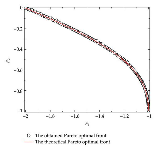
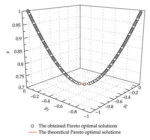
Example 4.1. Example 4.1 is taken from [22]. Here x ∈ R¹, y ∈ R². In this example, the population size and iteration times are set as follows: N_u = 200, T_u = 200, N_l = 40, T_l = 40, and T = 40:

()

Figure 1 shows the obtained Pareto front of this example by the proposed algorithm. From Figure 1, it can be seen that the obtained Pareto front is very close to the theoretical Pareto optimal front, and the average distance between the obtained Pareto optimal front and the theoretical Pareto optimal front is 0.00026, that is, GD = 0.00026 (see Table 2). Moreover, the lower SP value (SP = 0.17569, see Table 2) shows that the proposed algorithm is able to obtain a good distribution of solutions on the entire range of the theoretical Pareto optimal front. Figure 2 shows the obtained solutions of this example, which follow the relationship, that is, y₁ = −1 − y₂,

and

. It is also obvious that all obtained solutions are close to being on the upper level constraint G(x) boundary (1 + y₁ + y₂ = 0).

Table 2. Results of the Generation Distance (GD) and Spacing (SP) metrics for Examples 4.1 and 4.2.

Example	GD	SP
Example 4.1	0.00026	0.17569
Example 4.2	0.00004	0.00173

Details are in the caption following the image — **Figure 1**
Open in figure viewer PowerPoint

The obtained Pareto optimal front of Example 4.1.

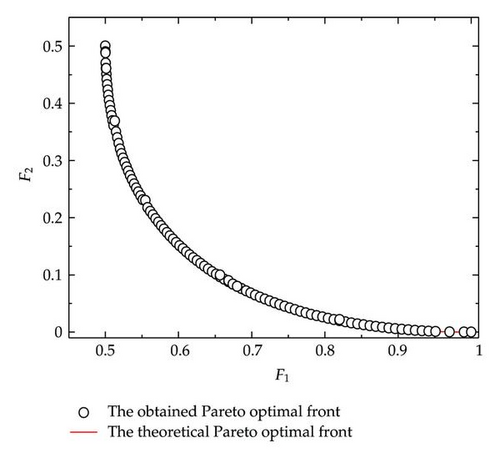
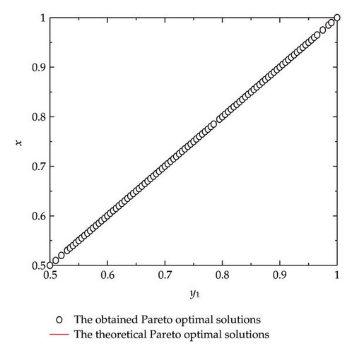
Example 4.2. Example 4.2 is taken from [36]. Here x ∈ R¹, y ∈ R². In this example, the population size and iteration times are set as follows: N_u = 200, T_u = 50, N_l = 40, T_l = 20, and T = 40.

()

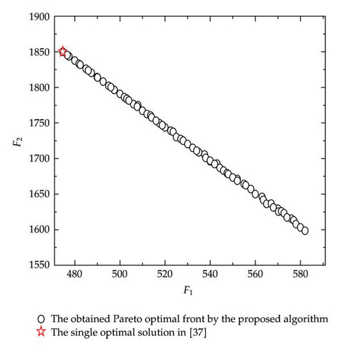
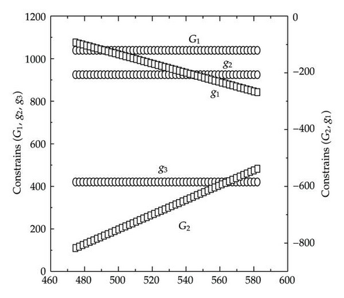
Figure 3 shows the obtained Pareto optimal front of this example by the proposed algorithm. From Figure 3, it is obvious that the obtained Pareto optimal front is very close to the theoretical Pareto optimal front, the average distance between the obtained Pareto optimal front and the theoretical Pareto optimal front is 0.00004 (see Table 2). On the other hand, the obtained Pareto optimal solutions can be distributed uniformly on entire range of theoretical Pareto optimal front based on the fact that the SP value is lower (SP = 0.00173, see Table 2). Figure 4 shows the obtained Pareto optimal solutions; they follow the relationship, that is, x = y₁, y₁ ∈ [0.5,1] and y₂ = 0.

Example 4.3. Example 4.3 is taken from [37], in which the theoretical Pareto optimal front is not given. Here x ∈ R², y ∈ R³. In this example, the population size and iteration times are set as follows: N_u = 100, T_u = 50, N_l = 20, T_l = 10, and T = 40:

()

Figure 5 shows the obtained Pareto optimal front of Example 4.3 by the proposed algorithm. Figure 6 shows all five constrains for all obtained Pareto optimal solutions and it can be seen that the G₁, g₂ and g₃ are active constrains. Note that, Zhang et al. [37] only obtained a single optimal solution x = (146.2955,28.9394), and y = (0,67.9318,0)which lies on the maximum of the F₂ using weighted sum method. In contrast, a set of Pareto optimal solutions is obtained by the proposed algorithm. However, the fact that the single optimal solution in [37] is included in the obtained Pareto optimal solutions illustrates the feasibility of proposed algorithm.

5. Conclusion

In this paper, an improved PSO is presented for BLMPP. The BLMPP is transformed to solve the multiobjective optimization problems in the upper level and the lower level interactively using the proposed algorithm for a predefined count. And a set of accurate Pareto optimal solutions for BLMPP is obtained by the elite strategy. The experimental results illustrate that the obtained Pareto front by the proposed algorithm is very close to the theoretical Pareto optimal front, and the solutions are also distributed uniformly on entire range of the theoretical Pareto optimal front. Furthermore, the proposed algorithm is simple and easy to implement. It also provides another appealing method for further study on BLMPP.

Acknowledgment

This work is supported by the National Science Foundation of China (71171151, 50979073).

References

1 Colson B., Marcotte P., and Savard G., An overview of bilevel optimization, Annals of Operations Research. (2007) 153, 235–256, https://doi.org/10.1007/s10479%2D007%2D0176%2D2, 2329985, ZBL1159.90483.
10.1007/s10479-007-0176-2
Web of Science® Google Scholar
2 Vicente L. N. and Calamai P. H., Bilevel and multilevel programming: a bibliography review, Journal of Global Optimization. (1994) 5, no. 3, 291–306, https://doi.org/10.1007/BF01096458, 1299018, ZBL0822.90127.
10.1007/BF01096458
Web of Science® Google Scholar
3 Bard J. F., Practical Bilevel Optimization: Algorithms and Applications, 1998, 30, Kluwer Academic, Dordrecht, The Netherlands, 1680111.
10.1007/978-1-4757-2836-1
Google Scholar
4 Dempe S., Foundations of Bilevel Programming, 2002, 61, Kluwer Academic, Dordrecht, The Netherlands, Nonconvex Optimization and its Applications, 1921449.
Web of Science® Google Scholar
5 Dempe S., Annotated bibliography on bilevel programming and mathematical programs with equilibrium constraints, Optimization. (2003) 52, no. 3, 333–359, https://doi.org/10.1080/0233193031000149894, 1996321, ZBL1140.90493.
10.1080/0233193031000149894
Web of Science® Google Scholar
6 Luo Z.-Q., Pang J.-S., and Ralph D., Mathematical Programs with Equilibrium Constraints, 1996, Cambridge University Press, Cambridge, UK, 1419501.
10.1017/CBO9780511983658
Google Scholar
7 Shimizu K., Ishizuka Y., and Bard J. F., Nondifferentiable and Two-Level Mathematical Programming, 1997, Kluwer Academic, Dordrecht, The Netherlands, 1429865.
10.1007/978-1-4615-6305-1
Google Scholar
8 Colson B., Marcotte P., and Savard G., Bilevel programming: a survey, Quarterly Journal of Operations Research. (2005) 3, no. 2, 87–107, https://doi.org/10.1007/s10288%2D005%2D0071%2D0, 2156141, ZBL1134.90482.
10.1007/s10288-005-0071-0
Google Scholar
9 Wang G. M., Wan Z. P., and Wang X. J., Bibliography on bilevel programming, Advances in Mathematics. (2007) 36, no. 5, 513–529, 2380906.
Google Scholar
10 Vicente L. N. and Calamai P. H., Bilevel and multilevel programming: a bibliography review, Journal of Global Optimization. (1994) 5, no. 3, 291–306, https://doi.org/10.1007/BF01096458, 1299018, ZBL0822.90127.
10.1007/BF01096458
Web of Science® Google Scholar
11 Wen U. P. and Hsu S. T., Linear bi-level programming problems. A review, Journal of the Operational Research Society. (1991) 42, no. 2, 125–133, 2-s2.0-0026103971, ZBL0722.90046.
Web of Science® Google Scholar
12 Koh A., Solving transportation bi-level programs with differential evolution, Proceedings of the IEEE Congress on Evolutionary Computation (CEC ′07), September 2007, 2243–2250, 2-s2.0-40649118020, https://doi.org/10.1109/CEC.2007.4424750.
10.1109/CEC.2007.4424750
Google Scholar
13 Mathieu R., Pittard L., and Anandalingam G., Genetic algorithm based approach to bilevel linear programming, RAIRO Recherche Opérationnelle. (1994) 28, no. 1, 1–21, 1269099, ZBL0857.90083.
10.1051/ro/1994280100011
Web of Science® Google Scholar
14 Oduguwa V. and Roy R., Bi-level optimization using genetic algorithm, Proceedings of the IEEE International Conference on Artificial Intelligence Systems, 2002, 322–327.
Google Scholar
15 Wang Y., Jiao Y. C., and Li H., An evolutionary algorithm for solving nonlinear bilevel programming based on a new constraint-handling scheme, IEEE Transactions on Systems, Man and Cybernetics Part C. (2005) 35, no. 2, 221–232, 2-s2.0-18544384528, https://doi.org/10.1109/TSMCC.2004.841908.
10.1109/TSMCC.2004.841908
Google Scholar
16 Yin Y., Genetic-algorithms-based approach for bilevel programming models, Journal of Transportation Engineering. (2000) 126, no. 2, 115–119, 2-s2.0-0034156245, https://doi.org/10.1061/(ASCE)0733%2D947X(2000)126:2(115).
10.1061/(ASCE)0733-947X(2000)126:2(115)
Web of Science® Google Scholar
17 Shi X. and Xia H., Interactive bilevel multi-objective decision making, Journal of the Operational Research Society. (1997) 48, no. 9, 943–949, 2-s2.0-0031233244, ZBL0892.90200.
10.1057/palgrave.jors.2600435
Web of Science® Google Scholar
18 Shi X. and Xia H., Model and interactive algorithm of bi-level multi-objective decision-making with multiple interconnected decision makers, Journal of Multi-Criteria Decision Analysis. (2001) 10, 27–34, https://doi.org/10.1002/mcda.285, ZBL0985.90054.
10.1002/mcda.285
Google Scholar
19 Abo-Sinna M. A. and Baky I. A., Interactive balance space approach for solving multi-level multi-objective programming problems, Information Sciences. (2007) 177, no. 16, 3397–3410, 2-s2.0-34249659575, https://doi.org/10.1016/j.ins.2007.02.005.
10.1016/j.ins.2007.02.005
Web of Science® Google Scholar
20 Nishizaki I. and Sakawa M., Stackelberg solutions to multiobjective two-level linear programming problems, Journal of Optimization Theory and Applications. (1999) 103, no. 1, 161–182, https://doi.org/10.1023/A:1021729618112, 1714988, ZBL0945.90057.
10.1023/A:1021729618112
Web of Science® Google Scholar
21 Zheng Y., Wan Z., and Wang G., A fuzzy interactive method for a class of bilevel multiobjective programming problem, Expert Systems with Applications. (2011) 38, 10384–10388, https://doi.org/10.1016/j.eswa.2011.02.069.
10.1016/j.eswa.2011.02.069
Web of Science® Google Scholar
22 Eichfelder G., Solving nonlinear multi-objective bi-level optimization problems with coupled upper level constraints, Technical Report, 2007, no. 320, Institute of Applied Mathematics, University Erlangen-Nrnberg, Germany.
Google Scholar
23 Eichfelder G., Multiobjective bilevel optimization, Mathematical Programming. A Publication of the Mathematical Programming Society. (2010) 123, no. 2, 419–449, https://doi.org/10.1007/s10107%2D008%2D0259%2D0, 2595920, ZBL1198.90347.
10.1007/s10107-008-0259-0
Web of Science® Google Scholar
24 Deb K. and Sinha A., Constructing test problems for bilevel evolutionary multi-objective optimization, Proceedings of the IEEE Congress on Evolutionary Computation (CEC ′09), May 2009, 1153–1160, 2-s2.0-70449838803, https://doi.org/10.1109/CEC.2009.4983076.
10.1109/CEC.2009.4983076
Google Scholar
25 Deb K. and Sinha A., Solving bilevel multiobjective optimization problems using evolutionary algorithms, 5467, Proceedings of the 5th International Conference on Evolutionary Multi-Criterion Optimization (EMO ′09), 2009, 110–124, Lecture Notes in Computer Science.
Google Scholar
26 Deb K. and Sinha A., An evolutionary approach for bilevel multiobjective problems, Cutting-Edge Research Topics on Multiple Criteria Decision Making, 2009, 35, Berlin, Germany, 17–24, Communications in Computer and Information Science, https://doi.org/10.1007/978%2D3%2D642%2D02298%2D2_3.
10.1007/978-3-642-02298-2_3
Google Scholar
27 Sinha A. and Deb K., Towards understanding evolutionary bilevel multiobjective optimization algorithm, Technical Report, 2008, no. 2008006, Department of Mechanical Engineering, Indian Institute of Technology Kanpur, Kanpur, India.
Google Scholar
28 Deb K. and Sinha A., An efficient and accurate solution methodology for bilevel multi-objective programming problems using a hybrid evolutionary local-search algorithm, Technical Report, 2009, no. 2009001.
Google Scholar
29 Sinha A., [email protected], Bilevel multi-objective optimization problem solving using progressively interactive EMO, 6576, Proceedings of the 6th International Conference on Evolutionary Multi-Criterion Optimization (EMO ′11), 2011, 269–284, https://doi.org/10.1007/978%2D3%2D642%2D19893%2D9_19.
10.1007/978-3-642-19893-9_19
Google Scholar
30 Kennedy J., Eberhart R., and Shi Y., Swarm Intelligence, 2001, Morgan Kaufmann, San Francisco, Calif, USA.
Google Scholar
31 Li X., [email protected], Tian P., and [email protected], Min X., [email protected], A hierarchical particle swarm optimization for solving bilevel programming problems, 4029, Proceedings of the 8th International Conference on Artificial Intelligence and Soft Computing (ICAISC ′06), 2006, 1169–1178, Lecture Notes in Computer Science, https://doi.org/10.1007/11785231_122.
10.1007/11785231_122
Google Scholar
32 Kuo R. J. and Huang C. C., Application of particle swarm optimization algorithm for solving bi-level linear programming problem, Computers & Mathematics with Applications. (2009) 58, no. 4, 678–685, https://doi.org/10.1016/j.camwa.2009.02.028, 2554011, ZBL1189.90212.
10.1016/j.camwa.2009.02.028
Web of Science® Google Scholar
33 Gao Y., Zhang G., Lu J., and Wee H. M., Particle swarm optimization for bi-level pricing problems in supply chains, Journal of Global Optimization. (2011) 51, 245–254, 2-s2.0-77956384018, https://doi.org/10.1007/s10898%2D010%2D9595%2D8.
10.1007/s10898-010-9595-8
Web of Science® Google Scholar
34 Deb K., Pratap A., Agarwal S., and Meyarivan T., A fast and elitist multiobjective genetic algorithm: NSGA-II, IEEE Transactions on Evolutionary Computation. (2002) 6, no. 2, 182–197, 2-s2.0-0036530772, https://doi.org/10.1109/4235.996017.
10.1109/4235.996017
Web of Science® Google Scholar
35 Deb K., Multi-objective optimization using evolutionary algorithms, IEEE Transactions on Evolutionary Computation. (2002) 6, 182–197, https://doi.org/10.1109/4235.996017.
10.1109/4235.996017
Web of Science® Google Scholar
36 Deb K. and Sinha A., Solving bilevel multi-objective optimization problems using evolutionary algorithms, Kangal Report, 2008.
Google Scholar
37 Zhang G., Liu J., and Dillon T., Decentralized multi-objective bilevel decision making with fuzzy demands, Knowledge-Based Systems. (2007) 20, 495–507, https://doi.org/10.1016/j.knosys.2007.01.003.
10.1016/j.knosys.2007.01.003
Web of Science® Google Scholar

Citing Literature

All articles

An Improved Particle Swarm Optimization for Solving Bilevel Multiobjective Programming Problem

Abstract

1. Introduction

2. Problem Formulation