The estimation of ground subsidence processes is an important subject for the asset management of civil infrastructures on soft ground, such as airport facilities. In the planning and design stage, there exist many uncertainties in geotechnical conditions, and it is impossible to estimate the ground subsidence process by deterministic methods. In this paper, the sets of sample paths designating ground subsidence processes are generated by use of a one-dimensional consolidation model incorporating inhomogeneous ground subsidence. Given the sample paths, the mixed subsidence model is presented to describe the probabilistic structure behind the sample paths. The mixed model can be updated by the Bayesian methods based upon the newly obtained monitoring data. Concretely speaking, in order to estimate the updating models, Markov Chain Monte Calro method, which is the frontier technique in Bayesian statistics, is applied. Through a case study, this paper discussed the applicability of the proposed method and illustrated its possible application and future works.

1. Introduction

In Japan, it is not rare to build airports on man-made islands or reclamation land. In these offshore airports, the airport pavement may be damaged due to the ground’s inhomogeneous subsidence. If the performance standard regarding airport pavement gradients is not satisfied, due to the progression of ground subsidence, large-scale repair work on concrete pavement is necessary. Therefore, predicting future ground subsidence is an important issue for asset management strategy of airport pavements.

Ground subsidence estimation models using the consolidation theory have been developed for soft ground [1]. However, there are many uncertainties in the actual ground conditions, and it is extremely difficult to deterministically predict the process of ground subsidence. Therefore, a method of probabilistically predicting the process of ground subsidence using a one-dimensional consolidation model that takes inhomogeneous subsidence into consideration, and using soil constants that show ground conditions as random variables, was developed [2]. With these probabilistic ground subsidence models, soil constants are generated with Monte Carlo simulation, and sample paths of the process of ground subsidence are simulated in accordance.

In this paper, a statistical ground subsidence model (hereinafter, mixed ground subsidence model) is expressed as the aggregation of sample paths sought by probabilistic ground subsidence models. Then, a mixed ground subsidence model, which employs monitoring information of ground subsidence after the establishment of airports, and sequentially performs Bayesian updating on weight coefficients of sample paths, is proposed. With this method, the accuracy of estimation of ground subsidence using monitoring information can be improved sequentially. The estimation accuracy of the mixed ground subsidence model depends on the method of generation of sample paths and its estimation accuracy.

With the above issues, this paper proposes a mixed ground subsidence model targeted for offshore airports. In the following sections, Section 2 organizes the basic idea of the study, Section 3 formulates a mixed ground subsidence model using the sample paths, Section 4 proposes a Bayesian updating model, and Section 5 introduces a numerical calculation example.

2. Basic Approach of This Study

2.1. Mixed Ground Subsidence Model

The target period is divided into two periods: before the airport was in service and after it began services. The former period shall be defined as the planning phase, and the latter the operating phase. For the planning phase, there is no monitoring information regarding ground subsidence process. Therefore, it becomes an issue to predict the amount of ground subsidence over the years for each mesh, using the first model (probabilistic one-dimensional consolidation model). The airport manager performs necessary boring tests during the planning phase and acquires data on ground subsidence. Data acquired by boring tests is partial information regarding ground subsidence, and not complete information. Therefore, the process of ground subsidence cannot be definitely predicted. Consequently, for the planning phase, several scenarios of ground subsidence will be established and sample paths of ground subsidence process for each mesh will be acquired. Then, using the sample information, the statistical regularity of the process of ground subsidence is expressed using the second model. From the second model, it is possible to express the probabilistic distribution of the deterioration process. Next, the operating phase is considered. From the point when the airport begins services, the airport manager continuously monitors ground subsidence amount for each mesh. The airport manager uses the monitoring information of the ground subsidence amount to conduct Bayesian updating on the second model and formulates the third model. The ground subsidence estimation model proposed in this paper is a composite estimation model comprising the following: (1) the probabilistic one-dimensional consolidation model (first model) that generates sample paths of the ground subsidence process, (2) the mixed ground subsidence model (second model) that expresses the statistical regularity of the sample paths generated with the first model, and (3) the third model updated by Bayesian updating on the second model using new monitoring information acquired as time passes.

In this paper, the subsidence process of airport ground is expressed using a probabilistic one-dimensional consolidation model, with consideration to the process of inhomogeneous ground subsidence. Therefore, the targeted airport ground is divided into planar meshes and also uses a three-dimensional model that divides meshes perpendicular to each planar mesh. By using the first model, the change over time in the amount of ground subsidence can be predicted for each planar mesh. However, there are many uncertainties in ground conditions. Therefore, using a one-dimensional consolidation model with randomly sampled ground conditions, multiple ground subsidence scenarios will be generated. The ground condition of each three-dimensional mesh is established by random generation. If the ground condition of each mesh is established in this way, the ground subsidence process over time of each planar mesh can be predicted using the first model. A ground subsidence process obtained in this way is one sample of subsidence process (hereinafter, sample path) for that ground condition scenario by random generation.

By randomly generating ground condition scenarios, multiple sample paths can be obtained for each planar mesh. In order to develop an airport pavement design and maintenance plan, it is necessary to summarize the numerous sample path information created by the first model. The easiest method is to use an expectation path that averages the sample paths generated with the first model. An expectation path is convenient, but it does not adequately utilize the enormous information acquired by the first model. Therefore, in this paper, weight coefficients are assigned to the sample paths acquired by the first model, and a mixed ground subsidence model (second model) that expresses the ground subsidence process by weight average of the sample paths is formulated. As the actual ground subsidence process cannot be observed in the planning phase, it is impossible to statistically predict the second model. Thus, unless there is theoretical or experiential additional information on the certainty of each sample path, the weight of each sample path must be handled equally. In other words, the ground subsidence process is defined as the expectation path that averages all sample paths. However, after the airport begins services, monitoring information on the process of ground subsidence can be acquired. The issue now is to improve the estimation accuracy of the ground subsidence process by using the monitoring information and sequentially performing Bayesian updating on the second model. The model acquired by Bayesian updating using monitoring information will be called the third model.

2.2. Bayesian Updating Scheme

In airport pavement management, it is required that the ground subsidence process is continuously monitored, the subsidence process predicted in the planning phase is reevaluated, and if necessary the maintenance strategy is reconsidered. As shown in Figure 1, let us say a certain amount of time has passed since the point when airport services began t₀ and has reached point T. The ground subsidence process is predicted during the planning phase with the probabilistic one-dimensional consolidation model. The dotted lines in the figure are the predicted results of the amount of ground subsidence over time, for a certain planar mesh. The figure shows sample paths of ground subsidence process for 20 calculation scenarios, with altered soil constants. Furthermore, the thick red line in the figure is the expectation path, which is the simple average of these paths. Let us say that after the airport begins services, the ground subsidence process of each mesh is continuously monitored. In the figure, the ground subsidence amount actually observed from point t₀ when services began and the current point T is shown with the black dots. In this example, the actual values of the ground subsidence are in a lower position than the expectation path. Therefore, when ground subsidence is predicted using the expectation path, the actual subsidence may be underestimated.

Details are in the caption following the image — **Figure 1**
Open in figure viewer PowerPoint

Bayesian updating on mixed ground subsidence model.

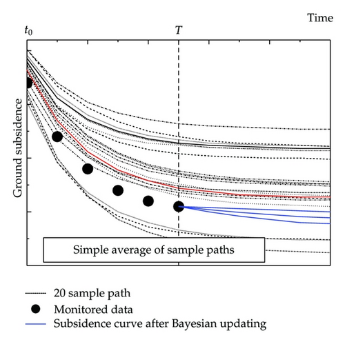
The mixed ground subsidence model can be obtained by assigning weight coefficients to sample paths and seeking the weight average of sample paths. Furthermore, let us say the distribution is according to prior distribution with weight vectors. At the initial point there is no monitoring information regarding ground subsidence. Therefore, equal weight is assigned to all sample paths. However, when monitoring information is acquired, higher weight can be assigned to sample paths closer to the observed values of ground subsidence amount. As a result, it is possible to limit the distribution range of weight coefficients within a narrower range. In Figure 1, the ground subsidence sample paths predicted for after point T are shown in thick blue lines, using the mixed ground subsidence model with Bayesian updating with monitoring information up to point T. In comparison to the spread of the sample paths sought with the first model, sample paths with Bayesian updating are collected within a narrower range, and it can be understood that the estimation accuracy of the mixed ground subsidence model is improved.

3. Mixed Ground Subsidence Model

3.1. Purpose of Second Model

By using the first model, sample paths regarding multiple ground subsidence processes can be generated for each planar mesh. In other words, each sample path shows the result of ground subsidence process simulation, with randomly generated soil constants as conditions. There are many uncertainties with ground conditions, so there is no guarantee that the actually observed ground subsidence process matches one sample path. In this chapter, the actual ground subsidence process is expressed with a mixed ground subsidence model, which expresses the aggregation of sample paths obtained with the first model. As mentioned above, the expectation path is the expectation sought from all sample paths and can be said to be a special case of the mixed ground subsidence model with equal weight assigned to all sample paths. Using the mixed ground subsidence model (second model), it is possible to express the probabilistic structure behind the sample paths. Furthermore, merits of the second model include (1) Bayesian updating of the ground subsidence model using monitoring information of ground subsidence amount observed at airports after services begin is made easy and (2) statistical testing on estimation accuracy of the ground subsidence model is possible.

3.2. Formalization of Mixed Ground Subsidence Model

The sample path k = 1, …, K calculated with the first model expresses the ground subsidence amount at point t for each mesh. The ground subsidence amount at point t (t = 0, …, T) in sample path k of planar mesh i (i = 1, …, N) can be expressed as f_i(t, k). The mixed ground subsidence model is defined as an aggregation of sample paths generated with the first model. For weight coefficients assigned to each sample path to be uniquely determined, the sample paths that comprise the mixed ground subsidence model must be independent. Let us say a total of K independent samples are obtained. The mixed ground subsidence model can be expressed as the linear combination of sample paths:

()

Here, ω_i(k) is the weight assigned to the sample path k, and the following holds:

()

Here, the weight vector of planar mesh i shall be expressed as ω_i = (ω_i(1), …, ω_i(K)). The weight vector ω_i is a random variable that satisfies the constrained condition (3.2). Next, let us assume that ε_i is a random variable that expresses the measurement error and each independently is subject to the one-dimensional normal distribution

3.3. Probabilistic Estimation of Ground Subsidence Amount

The weight matrix ω_i and probability error ε_i of the mixed ground subsidence model (3.1) are random variables. If these random variable values can be formalized, specific ground subsidence paths can be acquired. Here, let us say the prior probability density function of ω_i is subject to the Dirichlet distribution. The probability density function of the Dirichlet distribution is given by

()

Here, Γ(-) is a gamma function, and

is a constant parameter vector in the initial data. During the planning phase, the calculation results of the first model (sample paths) are available, as forerunning information [3]. The method of establishing parameters of the Dirichlet distribution using sample paths will be discussed in Section 5.3. Next, we will say

, and the prior probability density function of ϕ_i is subject to a gamma distribution. In other words, ϕ_i∽G(β⁽⁰⁾, γ⁽⁰⁾), and the probability density function of the gamma distribution is given by

()

Hence, β⁽⁰⁾ and γ⁽⁰⁾ are constant parameters in the initial data. At this time, the prior probability density function

of the ground subsidence amount

at point t of mesh i can be expressed as

()

However,

. It is difficult to analytically calculate the prior probability density function

, so it shall be calculated with Monte Carlo simulation. In other words, by random sampling ϕ_i, ω_i (1), …, ω_i (K − 1) with prior probability density functions (3.3a) and (3.4), and randomly selecting

with the normal probability density function

, the probability distribution of the ground subsidence amount can be estimated.

4. Bayesian Updating Model

4.1. Bayesian Updating of the Mixed Ground Subsidence Model

The mixed ground subsidence model is a statistical model that expresses statistical uncertainties in ground subsidence process, using sample paths of ground subsidence process generated by the first model. The mixed ground subsidence model includes random variables ω_i (weight vector assigned to each sample path) and ε_i (probabilistic error). At the initial point, measurement values for these random variables do not exist, and the statistical characteristics of the ground subsidence process is expressed with the random variables’ prior probability density functions (3.3a) and (3.4). In the operating phase when the airport is in service, monitoring information regarding the ground subsidence amount of each mesh is measured. Now, let us say time has passed from the point when services began (hereinafter, initial point) and has reached point T. Furthermore, let us say that from monitoring at point t (t = 0, …, T), the data regarding ground subsidence amount

has been acquired. The symbol “−” means the monitoring information (actual value). The overall monitoring results shall be expressed with the vector

. Here, let us consider for now that the weight vector ω_i is a given value, and only the probability error is a random variable. Also, the reciprocal ϕ of the probability error variance shall be a given value. Now, the likelihood that the monitoring result

is observed can be expressed as

()

Next, it shall be assumed that the prior probability density function of ω_i is subject to the Dirichlet distribution (3.3a), and the reciprocal ϕ_i of the variance follows the gamma distribution (3.4).

Here, the conditional posterior probability density function

of ϕ_i, with ω_i and

as known values, can be expressed as

()

In other words,

is subject to the gamma distribution

, and model samples of ϕ_i can be generated from the gamma distribution

Next, the conditional posterior probability density function

of ω_i, with ϕ_i and

as known values, can be expressed as

()

4.2. MH Algorithm

The conditional posterior probability density function of ω_i, shown in (4.3), is not a generally known distribution. Therefore, it is difficult to conduct direct sampling [4] of model samples of ω_i from the conditional posterior probability density function . This paper applies the MH (Metropolis-Hasting) method [5] that does not use a direct sampling method. The MH method samples from a proposed distribution that is similar to and according to it obtains samples from the original distribution [6]. Furthermore, to improve the efficiency of sampling, random walk is used. It is not new to use the MH method with random walk, but the algorithm should be explained briefly here, for the convenience of the reader.

First, the initial value of the parameter vector ω_i can be expressed as

. Here, a new candidate point

shall be proposed with

()

Here, λ is the constant parameter that establishes the range of step width, and ν = (ν(1), …, ν(K)) is the parameter vector that establishes the step width. In order for the candidate point

to satisfy the constrained condition

must hold. Now, from the change of variables ν^′ = ν + K⁻¹I, ν^′ shall be subject to the Dirichlet distribution. However, I is an identity matrix of 1 × K. The range of step width is the same for every k and established at (−λK⁻¹, λ(1 − K⁻¹)). Also, the proposed distribution shall be defined, using the Dirichlet distribution with the constant parameter vector x = (x₁, …, x_K), as follows:

()

This proposed distribution satisfies the condition:

()

Therefore, as the proposed density q is symmetrical to (

, the acceptance probability

of the new candidate point can be expressed as

()

If accepted, it moves to a new candidate point, and if rejected it remains. The MH algorithm procedure can be organized as follows.

Step 1 (Initial Establishment). The parameter vectors , and γ⁽⁰⁾ of the prior distributions (3.3a) and (3.4) are arbitrarily established. Furthermore, the initial values and of the parameter estimation are arbitrarily established. The constant parameter λ, constant parameter vector χ, and sample numbers and are established. The influence of these initial values shall decrease gradually, as the number of MCMC simulations increase. The number of simulations has to be n = 0.

Step 2 (Sample Extraction of Parameter Estimation ωi). The parameter estimation when the number of simulations is n + 1 is generated as follows. ν^′ that is subject to the Dirichlet distribution is randomly generated. The parameter vector ν that establishes the step width is calculated with ν = ν^′ − K⁻¹I. The new candidate point is

()

The acceptance probability is calculated as

()

Then the uniform distribution u ~ U(0,1) is generated, and if the two following equations are satisfied:

()

then

, so proceed to Step 3. If not, return to Step 2.

Step 3 (Sample Extraction of Parameter Estimation ϕi). is generated from . In other words, is randomly generated from the gamma distribution .

Step 4 (Final Judgment of the Algorithm). The updated values , of the parameter estimation, obtained from the above steps, are recorded. If , then n = n + 1 so return to Step 2. If not, the algorithm is finished.

4.3. Bayesian Updating and Bayesian Estimation

It shall be considered that using the monitoring result

of mesh i up to the monitoring at point t, the posterior distribution of the unknown parameters of the mixed ground subsidence model is obtained. Then, using the monitoring result

from between point t + 1 and t^′, the problem of updating the posterior distribution of the unknown parameters is supposed. If the posterior probability density function of the unknown parameters of the first Bayesian estimation is

, the posterior probability density function of the unknown parameter after the second Bayesian updating

can be expressed as

()

Here,

is the likelihood function defined using the database that pools the monitoring results from the initial point to point t^′. On the other hand, D(ω_i∣α⁽⁰⁾) and g(ϕ_i∣β⁽⁰⁾, γ⁽⁰⁾) are each prior distributions of ω_i and ϕ_i used in the first Bayesian estimation. Therefore, the posterior distribution after Bayesian updating is

()

In other words, in order to update the posterior distribution of unknown parameters, it is necessary to define the likelihood functions with the database that includes new monitoring results and newly estimate the posterior distribution by the MH method.

The monitoring information

from initial point t = 0 to point t = T and the posterior distribution of the parameter of the mixed ground subsidence model

are assumed to be given values. With this, the ground subsidence amount after point t = T can be estimated. The actual value (monitoring information) of ground subsidence amount of planar mesh i at point t = T shall be expressed as

. On the other hand, the predicted value of ground subsidence amount for point

(>T), which comes after point t = T, predicted at point t = T, shall be

. If it is assumed that with the passing of time ground subsidence always progresses, then the following holds:

()

Hence, n is a natural number. Here, the parameter ω_i of the mixed ground subsidence model is a given value. At this time, if ground subsidence amount

is observed at point t = T, prediction residual of the mixed ground subsidence model can be expressed as

()

Furthermore, if the weight coefficient ω_i is given, the predicted value of ground subsidence amount at point

(>T), which comes after point t = T, predicted at point T, can be expressed definitely with the mixed ground subsidence model:

()

Next, the posterior distribution

of parameter ω_i updated by Bayesian updating using the monitoring information

up to point t = T can be approximated with MCMC method. Furthermore, the weight sample generated with MCMC method can be expressed as

. At this point, if ground subsidence amount

is observed at point T, the probability distribution function

regarding ground subsidence amount

at point

(>T) can be expressed as

()

However,

is the predicted value of ground subsidence for point

(>T), predicted at point T, using the weight coefficient sample value

, and can be defined as

()

Furthermore, the expected value of ground subsidence amount

at point

can be expressed as

()

Also, the 100% (1 − 2δ) credible interval of ground subsidence amount

of point

, predicted at point T, can be defined as

using sample order statistics

and

()

5. Empirical Study

5.1. Summary of Applied Case

In this paper, the offshore H airport is targeted. At this airport, with approximately 30 thousand commissions of short-range international passenger flights and commissions of international cargo flights during late-night and early-morning hours, PFI is applied from planning and construction to maintenance of basic facilities including aprons, airport safety facilities, supplementary facilities, roads and parking spaces, and green tracts. Among these, aprons are areas where aircraft are parked, and concrete pavement is used because of the necessity of strong resistance of fluidity and oil. These aprons are situated on soft ground, and the fatigue and deterioration of the concrete pavement due to inhomogeneous subsidence of the ground is a problem.

The targeted area was the apron area of H airport, with a range of 825 m × 400 m, and for consolidation subsidence the basic unit was a 25 m × 25 m square mesh. The apron area was divided into planar meshes. Also, the targeted consolidation layers were alluvial clay layer around GL-7 m to GL-25 m and diluvial clay layer around GL-25 m to GL-60 m, and the one-dimensional consolidation theory was used. With Markov hazard model [7], the correlation between soil constants can be considered. In this applied case, from the boring test results, the horizontal correlation length was set at b = 100 m, and the perpendicular correlation length was set at 4-5 m. The perpendicular mesh divisions were divided at every 4 m, even within the same ground. For analysis, from the 17 boring results and consolidation test results conducted on the targeted area, the alluvial clay layer and diluvial clay layer was divided in the depth direction into 10 layers, A_c1–A_c6 and D_c1–D_c4, respectively, and the soil constants were organized. Table 1 shows the inhomogeneous subsidence simulation soil constant used in the applied case.

Table 1. Soil constants using first model.

Compression index: C_c	Normal distribution
Initial void ratio e₀	Normal distribution
Consolidation yielding stress: P_c	Normal distribution
Consolidation coefficient: c_v	Log-normal distribution

5.2. Analysis Results by the First Model

The inhomogeneous subsidence shall be simulated with the first model. For each block, the soil constant is randomly generated from the probability distribution. Specifically, the soil constants of each consolidation layer divided perpendicularly were generated from the expected value, standard deviation, and coefficient of variation shown in Table 2, by normal distribution for compression index C_c, initial void ratio e₀, and consolidation yielding stress p_c, and by log-normal distribution for consolidation coefficient c_ν. Furthermore, these expected values and distributions are established according to boring test results conducted on representative planar meshes. For all three-dimensional blocks, the soil constants were randomly generated by the Monte Carlo simulation. The pairs of soil constants generated for all three-dimensional blocks shall be called calculation scenarios. Furthermore, for each calculation scenario, the ground subsidence process of the targeted calculation scenario is calculated with the first model.

Table 2. Soil constants for inhomogeneous subsidence simulation.

Layer	C_c (kN/m²)		e₀		p_c (kN/m²)		c_v (cm²/day)
Layer	EV	SD	EV	SD	EV	CV	EV	log c_v	log c_v SD
A_c1	0.45	0.07	1.34	0.17	70	0.36	993	−4.26	0.29
A_c2	0.41	0.06	1.21	0.11	59	0.33	1025	−4.15	0.09
A_c3	0.73	0.11	1.84	0.22	95	0.49	759	−4.40	0.33
A_c4	0.87	0.08	2.09	0.15	90	0.39	787	−4.32	0.23
A_c5	0.74	0.21	1.91	0.39	99	0.44	1103	−4.20	0.26
A_c6	0.31	0.12	1.17	0.22	139	0.08	3435	−3.63	0.09
D_c1	0.44	0.13	1.32	0.30	174	0.71	1680	−3.95	0.14
D_c2	0.57	0.16	1.54	0.27	144	0.67	1945	−4.01	0.34
D_c3	0.66	0.12	1.58	0.19	135	0.66	1000	−4.27	0.29
D_c4	0.70	0.25	1.64	0.67	186	0.65	1002	−4.23	1.66

Note—EV: expected value, SD: standard deviation, CV: coefficient of variation. For A_c1–A_c6, the alluvial clay ground layer was divided into 6 layers in the depth direction from categorization of soil characteristics, acquired from boring test results and lab consolidation test results, and the layers were numbered from the top layer to the bottom layer. Similarly, for D_c1–D_c4 also, according to the categorization of soil characteristics, the diluvial clay ground layers were numbered from the top layer to the bottom layer.

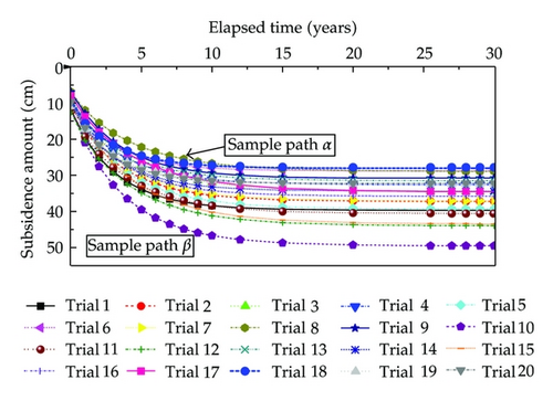
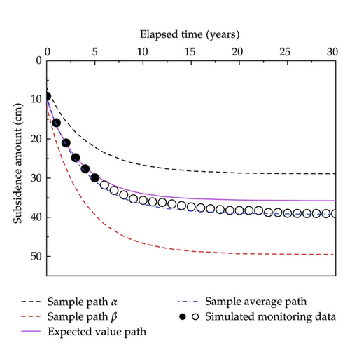
An example of the inhomogeneous subsidence simulation is shown in Figure 2. This figure shows 20 sample paths of ground subsidence amount over time, for the planar mesh i = 73, which was chosen as an example. The chosen planar mesh has an existing ground height of AP + 3.0 m, a planned ground height of AP + 6.0 m, and is a part of the area with high embankment. As a result of simulation with the first model, the expected path subsidence amount after 30 years is 35.75 cm as shown in Figure 3 and is predicted to have the largest subsidence among the entire targeted area. In the horizontal axis, the start of services at H airport is set at 0, but it can be seen that ground subsidence had already occurred between roadbed adjustment and the start of services. Also, when comparing the 20 sample paths of Figure 2, it can be understood that the ground subsidence amount changes greatly depending on the soil constant scenario. In fact the average subsidence amount for after 30 years is 35.75 cm and the variance is 30.66 cm². On the other hand, in any sample path the ground subsidence processes converge with the passing of time.

5.3. Creating the Second Model

Using the 20 sample paths obtained with the first model (see Figure 2), the mixed ground subsidence model (second model) is estimated. The sample paths from the first model are in a strong correlation to each other. For example, the correlation coefficient between the 20 sample paths of Figure 2 was at least 0.976. Therefore, in order to avoid the problem of multicollinearity, out of the 20 sample paths the 2 sample paths that set the upper limit and lower limit of predicted subsidence at the end of the contract were selected for the estimation of the mixed ground subsidence model. Hereinafter, the sample path at the upper limit shall be called α and the sample path at the lower limit shall be called β. We shall add that with any mesh, the sample path α and β set the upper and lower limits of predicted subsidence for the overall contract period. In other words, by selecting sample paths α and β, it is possible to expand the section between the two sample paths as much as possible and maximize the range created with the second and third models. Figure 3 shows the expected value path by simple average of the 20 sample paths. This figure also shows the averaged results of the 2 sample paths used for the mixed ground subsidence model (sample average). Naturally, this path does not match the expected value path, which is a simple average of the 20 sample paths. Therefore, in order to predict the ground subsidence amount

of mesh i at point t, the weight coefficient ω_i(k) (k = 1,2) of the mixed ground subsidence model must be corrected so that the misfit between the expected path of the mixed ground subsidence model and the sample average is as little as possible. Now, the predicted ground subsidence amount of mesh i at point t of the expected value path from the 20 sample paths shall be expressed as

. If ω_i(k) (k = 1,2) takes a value that satisfies:

()

then the misfit between the expected value path and average path is arbitrarily small. However, f_i(t, k) is the sample path (generated with the first model) selected for the mixed ground subsidence model. Now, the weight vector ω_i at point t established in (5.1) shall be expressed as

. Furthermore, let us say the prior probability density function of the weight vector ω_i of the mixed ground subsidence model can be identified as a Dirichlet distribution of (3.3a). The posterior probability density function

of ground subsidence amount

at point t of mesh i is difficult to analytically estimate as shown in (3.5), so it is necessary to calculate this with Monte Carlo simulation. For this, the weight vector ω_i is randomly generated from a Dirichlet distribution as shown in (3.3a). Therefore, in order to make the separation between the expected value path and average path arbitrarily small, a Dirichlet distribution and parameter vector is established in which the following equation approximately holds:

()

Now, in the Dirichlet distribution, the expected value of ω_i(k) can be expressed as

()

Therefore, the initial parameter of the Dirichlet distribution

is established so that the following holds:

()

Using the mixed ground subsidence model established with the above, the ground subsidence amount after 5 years

is predicted. The distribution of the predicted subsidence amount can be obtained, as shown in (3.5), by establishing the prior probability density function of α⁽⁰⁾ and ϕ_i. Now, the parameter vector of the Dirichlet distribution α⁽⁰⁾ shall be, according to the weight vector

, established as

and

. Figure 4 uses planar mesh i = 73 and shows how the predicted subsidence distribution changes after 5 years, due to the values of the parameters β⁽⁰⁾ and γ⁽⁰⁾ of the prior probability density function ϕ_i. As shown in Figure 4, if the values of parameters β⁽⁰⁾ and γ⁽⁰⁾ are increased, the predicted subsidence amount is distributed within a narrower range. On the other hand, if the values of β⁽⁰⁾ and γ⁽⁰⁾ are decreased, the predicted subsidence amount is distributed within a wider range. Figure 5 shows how the 95% credible interval of the predicted subsidence amount at point t changes according to the values β⁽⁰⁾ and γ⁽⁰⁾. The initial parameter of the prior probability density of ϕ_i can be arbitrarily established, but for the efficiency of Bayesian learning it is better if the prior distribution is dispersed. In this paper, the initial parameters were established at β⁽⁰⁾ = 0.5 and γ⁽⁰⁾ = 0.5. From the results of Figure 4, the case in which these initial values were used shows greater dispersion of prior distribution of the parameter values, among the 4 calculation cases in the same figure.

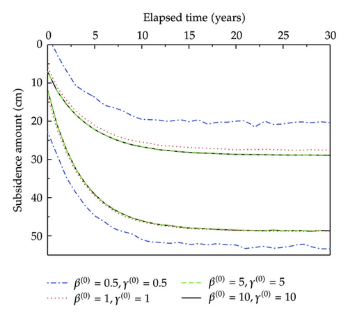
5.4. Estimating the Third Model

After services are offered at the airport, information on the ground subsidence amount of each planar mesh can be obtained through continuous monitoring. Using this monitoring information, the mixed ground subsidence model is reconsidered. At the moment, the airport is not in service and there is no monitoring information. So, the monitoring results of ground subsidence amount of each planar mesh are assumed and Bayesian updating is conducted on the mixed ground subsidence model. Now, the period of the airport during operation and management shall be divided into two periods: (1) from the first year to the sixth year and (2) after the sixth year. After services begin, each year periodical monitoring of ground subsidence amount is conducted, and at the fifth year after services begin, Bayesian estimation of the mixed ground subsidence model is considered. Next, after the sixth year, monitoring information of ground subsidence can be obtained each year. Here we shall consider the problem of adding the newly acquired monitoring information to the database and conducting Bayesian updating of the mixed ground subsidence model every year according to the newly updated database.

In the targeted airport ground, there are a total of 528 planar meshes. Let us assume the airport apron has been in service for 5 years, and consider the problem of predicting ground subsidence amount after the sixth year, using monitoring information of 5 years to update the mixed ground subsidence model. Figure 3 shows the sample path created with the first model and expected value path calculated with the second model, using an example mesh (i = 73) of the 528 planar meshes. Currently, there is no monitoring information so the Bayesian updated third model is created using assumed information. In order to check whether the estimation results of ground subsidence can be appropriately corrected with the Bayesian updated third model, even if the actual ground subsidence amount is larger than the expected path of the second model, the hypothesized monitoring information shown with the black dots in Figure 3 was used. The ground subsidence process shown in this example is lower than the expected sample path, and the ground subsidence amount is larger than the expected value path. The mixed ground subsidence model of the targeted mesh can be expressed as

()

Also, k = 1 is the sample path α of Figure 3, while k = 2 is sample path β.

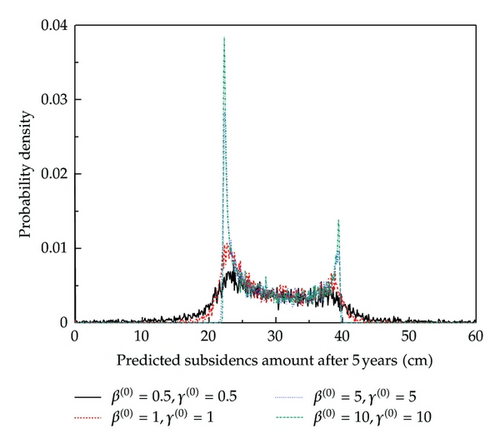
Furthermore, for the prior probability density function of weight vector ω_i of the mixed ground subsidence model, the same distribution was used as the Dirichlet distribution used in the second model. On the other hand, the prior probability density function of the variance parameter ϕ_i of the probability error term ε_i is subject to the gamma distribution of (3.4), and the parameter of the gamma distribution was established as (β⁽⁰⁾, γ⁽⁰⁾) = (0.5,0.5) according to the consideration of Section 5.3. Also, the number of convergence tests totaled 8,000 samples: .

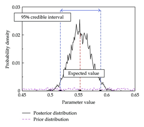
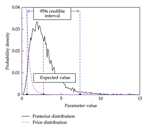
First, after services, the mixed ground subsidence model is updated with Bayesian updating according to the monitoring information of 5 years. In Table 3, the estimation results of the mixed ground subsidence model are shown with the weights ω₇₃(1), ω₇₃(2), expected value of distribution parameter ϕ₇₃, the 95% credible interval, and the Geweke test statistics [8]. Geweke test statistics are statistics for testing whether the sampling process of MCMC method reaches a steady state and is used to test whether the sample number is appropriate or not. From the estimation results, the total weight is 1 and the constrained condition equation (3.2) is satisfied. Also, the expected value of weight ω₇₃(1) is high but this is an inevitable result as the simulated monitoring information is at a higher position than the sample average path. The posterior probability density functions of these two parameters are shown in Figures 6 and 7. Also, when conducting the MH method, was established as the sample number for the Markov chain to reach a steady state, but the absolute value of the Geweke test statistics are all lower than 1.96 and the hypothesis that it “converges to a steady state” with a significance level of 5% cannot be dismissed. The prior distributions of these parameters are shown in Figures 6 and 7, but the variance of the parameter distributions of the mixed ground subsidence model is smaller with Bayesian updating.

Table 3. Estimation results of mixed ground subsidence model.

Parameter	Expected value	95% credible interval		Geweke test statistics
ω₇₃(1)	0.553	0.518	0.589	−8.63E − 02
ω₇₃(2)	0.447	0.428	0.467	−8.63E − 02
ϕ₇₃	2.76	0.66	7.41	−4.49E − 02

Next, using the mixed ground subsidence model updated with Bayesian updating on the fifth year, the ground subsidence path after the sixth year is estimated and the results are shown in Figure 8. As stated above, the actual path of ground subsidence process is simulated as having greater subsidence than the expected sample path. Therefore, the expected subsidence amount after 30 years has passed is 38.11 cm, 35.75 cm greater than the expected sample path. At year 30, the lower limit of the 95% credible interval is 37.99 cm and the upper limit is 38.22 cm, and it is understood that after Bayesian updating the estimation accuracy of the mixed ground subsidence model has improved and better risk management of ground subsidence is possible.

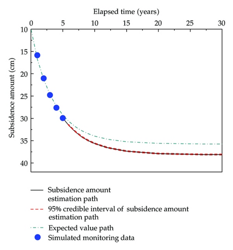
Furthermore, we shall consider how after the sixth year monitoring information is continuously accumulated and Bayesian updating is sequentially conducted on the mixed ground subsidence model. Let us look at planar mesh i = 73 once more. With this mesh, monitoring information as shown in the white dots in Figure 3 is accumulated after the sixth year. Here, let us say that as new monitoring information is obtained each year, Bayesian updating is conducted on the mixed ground subsidence model. Furthermore, using the updated mixed ground subsidence model, the ground subsidence amount at year 30 is estimated and the results are shown in Table 4. In this chart, using the mixed ground subsidence model after Bayesian updating with the monitoring information up to that point, the estimation (expected value) of the ground subsidence amount at the 30th year after being in service, as well as the upper and lower limits of the 95% credible interval, is shown. Furthermore, the simulated monitoring information (subsidence amount) at the 30th year is 39.09 cm. Compared to the Bayesian updating result, with the accumulation of information the expected path is slightly corrected and the credible interval range is narrower. From this it can be understood that the estimation accuracy is improved due to Bayesian updating.

Table 4. Estimation results of ground subsidence amount (mesh i=73).

Year	Subsidence estimation of 30th year	95% credible interval		Width of credible interval
5	38.109	37.990	38.224	0.234
6	38.209	38.139	38.279	0.140
7	38.218	38.174	38.263	0.089
8	38.226	38.199	38.254	0.055
9	38.439	38.419	38.457	0.038
10	38.151	38.140	38.163	0.023
15	38.115	38.114	38.116	0.002
20	38.477	38.477	38.477	0.000
25	39.046	39.046	39.046	0.000

Note: the simulated monitoring data (subsidence amount) at the 30th year is 39.09 cm.

6. Conclusion

This paper attempts to propose a methodology of conducting Bayesian updating on ground subsidence estimation results using continuous monitoring and monitoring information of ground subsidence, which is an important issue in asset management of airport facilities. Specifically, using a one-dimensional consolidation model that takes inhomogeneous subsidence into consideration, sample paths regarding ground subsidence process and a mixed ground subsidence model that averages the load of the sample paths are calculated. Furthermore, a methodology of conducting Bayesian updating using MCMC method on the mixed ground subsidence model, by continuously monitoring the ground subsidence amount after the airport begins services, is proposed. Furthermore, the applicability of the methodology proposed in this paper is empirically evaluated through an applied case of the ground subsidence estimation management of an airport facility. However, in order to improve the applicability of the Bayesian updating model proposed in this paper, there are several issues to be studied in the future. First, the applied case in this paper is at the state where the airport facilities have just begun services. Therefore, monitoring information is not yet available. Consequently, in the applied case, Bayesian updating of the mixed ground subsidence model was conducted using simulated monitoring information. In the future, it is necessary to continuously monitor the ground subsidence process of airports and use actual monitoring information to evaluate the efficiency of Bayesian updating on the mixed ground subsidence model. Secondly, in airport pavement management, ground subsidence estimation management is an important issue for consideration, but for pavement management, managing deterioration and damage processes of airport pavements is also important. For this, the deterioration and damage progress of airport pavements as well as ground subsidence should be modelized. Thirdly, the Bayesian updating model proposed in this paper is a methodology for conducting Bayesian updating on estimation results based on monitoring information during the designing phase. This type of Bayesian updating model has the potential to be applied to a wider range of problems outside of ground subsidence estimation management. In the future, it is necessary to evaluate the efficiency of the Bayesian updating model on asset management of public facilities other than airport pavements.

References

1 Tang W. H., Probabilistic evaluation of penetration resistances., Journal of the Geotechnical Engineering Division, ASCE. (1979) 105, no. 14902, 1173–1191, 2-s2.0-0018528922.
10.1061/AJGEB6.0000865
Web of Science® Google Scholar
2 Tsuchida T. and Ono K., Prediction of inhomogeneous subsidence based on numerical simulation and its application to design standard of airport pavement, The Port and Airport Research Institute Report. (1988) 27, no. 4, 123–200.
Google Scholar
3 Jeffreys H., Theory of Probability, 1961, Clarendon Press, Oxford, UK, 0187257, ZBL0116.34904.
Google Scholar
4 Gilks W. R. and Wild P., Adaptive rejection sampling for Gibbs sampling, Applied Statistics. (1992) 41, 337–348, https://doi.org/10.2307/2347565.
10.2307/2347565
Web of Science® Google Scholar
5 Ibrahim J. G., Chen M.-H., and Sinha D., Bayesian Survival Analysis, 2001, Springer, New York, NY, USA, Springer Series in Statistics, 1876598, ZBL1209.62036.
10.1007/978-1-4757-3447-8
Google Scholar
6 Kobayashi K., Kaito K., and Nam L. T., A bayesian estimation method to improve deterioration prediction for infrastructure system with markov chain model, International Journal of Architecture, Engineering and Construction. (2012) 1, no. 1, 1–13, https://doi.org/10.7492/IJAEC.2012.001.
10.7492/IJAEC.2012.001
CAS Google Scholar
7 Tsuda Y., Kaito K., Aoki K., and Kobayashi K., Estimating Markovian transition probabilities for bridge deterioration forecasting, Journal of Structural Engineering/Earthquake Engineering. (2006) 23, no. 2, 241s–256s, 2-s2.0-33847329274, https://doi.org/10.2208/jsceseee.23.241s.
10.2208/jsceseee.23.241s
Google Scholar
8 Geweke J., Evaluating the accuracy of sampling-based approaches to the calculation of posterior moments, Bayesian Statistics, 1996, 4, Oxford University Press, 169–193, 1380276.
Google Scholar

Citing Literature

All articles

A Mixed Prediction Model of Ground Subsidence for Civil Infrastructures on Soft Ground

Abstract

1. Introduction