Discrete Dynamics in Evolutionary Games
Abstract
This paper furnishes a guide for the study of 2-dimensional evolutionary games in discrete time. Evolutionarily stable strategies are identified and nonlinear outcomes are explored. Besides the baseline payoffs of the established strategic interaction, the following elements are also vital to determine the dynamic outcome of a game: the initial fitness of each agent and the rule of motion that describes how individuals switch between strategies. In addition to the dynamic rule commonly used in evolutionary games, the replicator dynamics, we propose another rule, which acknowledges the role of expectations and sophisticates the replicator mechanism.
1. Introduction
Evolutionary game theory addresses scenarios of strategic interaction in which players can switch between strategies over time following some dynamic adjustment process. As time passes by, strategies with higher associated payoffs will displace strategies with lower payoffs, under a process that is determined by some specified dynamic rule of evolution. In this type of setting, the most common result will be the convergence towards a dominant long-term outcome that eventually will end up by being followed by the whole of the universe of individuals in the considered population. Thus, we should expect to find an evolutionarily stable strategy (ESS), that is, the strategy, from the set of available strategies, that is robust to evolutionary pressures or the one that is uninvadable by any other strategy. The concept of ESS was first presented by Maynard-Smith and Price [1], who have launched the fruitful field of evolutionary game analysis. This field of knowledge may be interpreted as the science that studies the robustness of strategic behavior.
The idea of evolution in a strategic choice setting is powerful because it automatically questions the notion that agents act in a hyper-rational way. In evolutionary games there is an implicit recognition that agents learn: they begin by selecting a strategy, at time t = 0, that they do not know if it is the one that maximizes the corresponding utility. The systematic interaction with individuals selecting the same or other strategies will allow for an evaluation over time of what is the best choice to make. This is clearly a Darwinian environment—only the strongest strategies thrive and all the others will tend to disappear. The survival of the fittest requires individual agents to switch to the best strategy or, instead, to vanish from the game. This process occurs through interaction and experimentation. At the initial point in time, the agent does not know how the process will evolve, and therefore individual rationality is not vital to the final outcome. Instead, such outcome is shaped by natural selection, with fitter groups increasing their population shares at the expenses of less fit ones.
The initial approach to evolutionary games, due to Maynard-Smith [2], was essentially concerned with a long-run equilibrium analysis. The stability of the steady-state of the game was addressed, but the specific dynamic process conducting to the outcome remained without explicit specification. Taylor and Jonker [3] proposed a dynamic rule that is still today the most widely used to approach evolutionary games. This is the replicator dynamics, a rule according to which the share of agents following a given strategy increases with an above average fitness of the assumed strategy and diminishes in the opposite circumstance.
The typical approach to evolutionary game theory takes essentially two main components. First, a payoff matrix indicating the outcome of following a strategy, when the other agents follow the same or any other strategy, and, second, a dynamic rule, for example, the replicator dynamics. The initial setup was proposed for the interaction between animal species and it functioned as a powerful instrument to explain the evolution of species. The adaptation of the framework to other settings, particularly to social and economic contexts, requires a careful examination of the assumptions in which the paradigm of evolutionary interaction is founded; namely, the replicator dynamics is not a sufficiently general rule and the stability outcomes are conditioned by its specificity.
In this paper, we undertake a detailed analysis of the dynamics underlying evolutionary games in settings with two strategies. The study is developed in discrete time, in opposition to what is common in the evolutionary game theory literature, which generally takes a continuous time replicator dynamics equation. In discrete time, we will be able to identify nonlinear endogenous long-term outcomes, even in one-dimensional systems. Regular and irregular long-run endogenous fluctuations are meaningful because they imply that instead of converging to an ESS, the dynamics will lead to an everlasting movement through which part of the individuals will systematically switch between alternative strategies. There will not be a dominant strategy in the already mentioned uninvadable sense. Dynamics are analyzed first by considering the trivial replicator dynamic rule and, in a second moment, by taking a rule under which there is heterogeneity of access to relevant information by the agents in the population, which will also have different capabilities in what concerns the ability to accurately predict future scenarios.
The remainder of the paper is organized as follows. Section 2 makes a brief journey through the recent literature on evolutionary games, in order to identify the main applications (mostly in economics) that were built upon the theoretical principles of evolutionary games. Section 3 describes the generic framework of our simple evolutionary game. In Sections 4 and 5 we address stability properties under the selected evolutionary rules. Section 6 illustrates the dynamic outcomes with a series of examples, starting with the most common one, the Hawk-Dove game. Section 7 concludes.
2. Evolutionary Game Theory and Economic Thinking
The setup engineered by Maynard-Smith and Price [1] and Taylor and Jonker [3] has been extensively used to model economic issues in the last few years. As stated in the introduction, the original framework is not necessarily the most appropriate one to study economic phenomena, because it was prepared to analyze conflict in a biological context, a setting where evolutionary behavior dominates relatively to rational thinking. Evolution is a process according to which there is a natural movement in the direction of increased payoffs, because these are the ones allowing to obtain higher fitness. Economic processes have necessarily a component of evolution, but certain features of rational thinking must be considered as well. In this section, some of the adaptations of evolutionary game theory to economics are briefly discussed. This does not intend to be a thorough survey on this issue; for detailed discussions on evolutionary games and economic applications, see Weibull [4, 5], Vega-Redondo [6], and Friedman [7].
On general grounds, economists have tried to establish a link between the evolutionary process of strategy selection and the notion that economic equilibria is socially determined by the type of interaction that is established between agents in a society. According to M. G. Villena and M. J. Villena [8], in economics the evolutionary process will correspond to repeated interaction that leads to the formation of norms or institutions. As for the interaction within or among animal species, in society we can conceive a selection mechanism that favors some strategies over others; the strategies that perform better than average are the ones that become dominant in the long run. These dominant strategies will become the social norm, that is, the set of rules that are adopted by the majority of the population.
For Safarzyńska and van den Bergh [9], the introduction of the concept of evolution represents a relevant shift on economic thought, since many new dimensions gain visibility. Evolution occurs in a complex setting where the following ideas predominate: path-dependence and lock-in (outcomes are the result of concrete interaction situations that cannot be automatically reversed in time), bounded rationality (social norms are not chosen by a hyperrational agent; they are the result of interaction over time), diversity, innovation, selection, and diffusion (the choice of different strategies over time implies heterogeneity among individuals, the capacity to discover and select new paths, and some kind of diffusion process). The idea of looking at economic reality through the lenses of evolutionary selection of strategies, where boundedly rational players learn and in this way lead to the establishment of collective outcomes, has been emphasized as well by many other authors, for instance, Matsui [10], Sumaila and Apaloo [11], Josephson [12], Noailly et al. [13], Rota Bulò and Bomze [14], and Voelkl [15].
Most of the evolutionary interaction literature typically considers that an evolutionarily stable strategy is sooner or later attained. This result was first proved for the replicator dynamics, but it is extensive to other types of adjustment processes. Ponti [16] highlights that the replicator dynamics tends to generate a stability result because success breeds success, that is, a virtuous cycle is generated, according to which fitness results tend to increase every time the strategies with higher payoffs are chosen. Instead of considering a purely biological evolution mechanism, one can think of a process in which agents consider at the same time different ideas; these compete in their minds and which of them will predominate will depend on the experiences of the individuals. The notion that strategies compete in the minds of people as populations of ideas has been explored by Börgers and Sarin [17] and received the designation of reinforcement learning.
Although it may be the expected result, evolutionary interaction does not necessarily generate a stability outcome in which dominant strategies completely rule out dominated strategies. Hofbauer and Sandholm [18] study the scenarios in which dominated strategies may survive. The main argument in this reasoning relates to the idea that a disequilibrium result may subsist in the long term. Evolutionary dynamics need not converge and nonlinear endogenous results can eventually be obtained. Good current fitness might lead to the adoption of strategies that are good in the assumed time period but that are not optimal from an intertemporal point of view. This result was first noted by Skyrms [19], who pointed out that the long-term state is contingent on the type of dynamic rule that is considered. This author asks in which circumstances the equilibrium is not eventually reached and answers this question by exploring dynamic settings where complex nonconvergent behavior arises. In our paper, since we propose to address dynamics in discrete time, such type of nonlinear outcomes emerge even in one-dimensional dynamic systems.
- (1)
in a series of papers, Araújo [20], Araújo and de Souza [21], and Araújo et al. [22] study the dynamics of the labor market within an environment of evolutionary selection. Workers and firms choose between two strategies: to engage in business activities in the informal sector or in the formal sector of the economy. The evolutionary process implies, in this case, that there is not a unique possible solution; this will depend on the economy’s initial conditions and, therefore, at a given period the relative weight of the formal and informal sectors in the economy will be path dependent, that is, it will depend on the evolution of the interaction process so far;
- (2)
Gamba and Carrera [23] also study the interaction between firms and workers but from a different angle of analysis. In this case, firms select between the following strategies: to innovate or not to innovate (by investing or not in R&D). Workers choose whether to invest in human capital accumulation and, as a result, their choice is between being skilled or unskilled workers. In this case, decision making is determined by a replicator dynamics mechanism of evolution. The setting allows to address the presence of strategic complementarities between R&D and human capital;
- (3)
a setup where evolutionary game theory has also made a contribution is the one concerning public goods provision. In Clemens and Riechmann [24] and Antoci et al. [25], it is studied, under an evolutionary setting, a series of situations relating to the behavior of agents when asked to contribute to the provision of a public good. The available strategies involve voluntary contribution and free riding. Both strategies might eventually dominate the behavior in the population, depending on initial conditions, payoffs, and evolutionary rule;
- (4)
another type of game to which evolutionary theory may be adapted relates to macroeconomic monetary policy in the context of the Barro-Gordon policy choices game. In D’Artigues and Vignolo [26], two types of agents interact: the monetary authority and the private economy. The interaction process will shape the time trajectory of the inflation rate and the two possible long-term outcomes are states of low and high inflation;
- (5)
evolutionary games have also been applied in the field of neuroeconomics. Schipper [27] presents logical arguments in favor of evolving brains. Through interaction and strategy selection, the nervous system can develop in various ways, namely, it can converge to an equilibrium where it functions well;
- (6)
Kuechle [28] applies evolutionary game theory to explain the degree of entrepreneurial activity that tends to dominate in a society. Strategies involve engaging or not in entrepreneurship. Again, the setting is adequate since, as for other phenomena, we can interpret an equilibrium in this case as the result of finding a strategy that once adopted by a large fraction of the population it cannot be displaced by small groups of individuals adopting other kinds of behavior;
- (7)
in Hanauske et al. [29], evolutionary game theory is the tool used to address the behavior in financial markets. We know that financial markets are populated by heterogeneous agents, who adopt different kinds of beliefs on the functioning of the market. In particular, we can identify the presence of aggressive and nonaggressive agents. Aggressive behavior is characterized by investment in highly risky financial products that increase risk for the whole of the market, which leads to an increase in the probability of significant market crashes. Nonaggressive investors will be the ones endowed with higher levels of information, that is, the ones that will take a rational behavior given that they have good knowledge about market fundamentals. In an evolutionary game environment, the two types of agents interact and there is no reason to believe that nonaggressive behavior will necessarily be the prevailing long-term outcome, although aggressive behavior may result in an equilibrium with losses for the whole of the investors. Evolutionary game theory may provide, in this case, a result such that the ratio between aggressive and nonaggressive agents will converge to a stable steady-state fixed point. This fixed point will be determined by the expected losses and gains generated by the decisions of the agents in the context of interaction.
As emphasized by Guth [30], economics has a lot to gain with attempting to merge the traditional rational choice framework with the tradition in biology of assuming evolutionary processes that lead to results that are necessarily path dependent. Although evolutionary game theory has emerged essentially in the context of interaction between nonrational players, where choices are determined by past success, this is a powerful tool that is easily adaptable to scenarios of human interaction, where choices are made in the light of their future consequences. Behavior may be partially path dependent, but it also has a strong component of forward-looking deliberation. Applications to economics will require rules of adaptation that explicitly consider expectations.
3. Strategies, Payoffs, and Evolutionary Rules
The displayed aij values, i, j = 1,2, correspond to the payoffs of a player resorting to the strategy in the appropriate row, when matched with some player that adopts the strategy in the respective column.
Agents will end up by adopting the strategy for which the fitness value is larger.
The above equation indicates how the share of individuals on a population following strategy D evolves over time. Obviously, since only two strategies are considered, if we get to know the evolution of one of the shares, then we will also know how the other one behaves.
Because p∈[0,1], the following boundaries must apply to (3.5): if , then pt+1 = 0; if , then pt+1 = 1.
In Section 4, the dynamics underlying (3.5) will be thoroughly discussed. This allows to present results on long-run outcomes of the evolutionary process. The results will be contingent on the specific dynamic rule that was considered, namely, the replicator dynamics. In what follows, we propose an alternative rule.
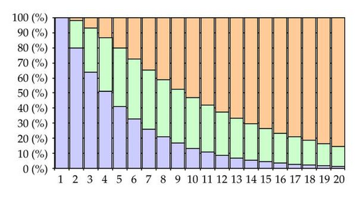
The three classes of more or less skillful agents coexist, in an environment with decreasing degrees of attentiveness. The first group dominates for expectations formed under a high degree of attentiveness; the last class, the less prepared to generate expectations and therefore the one resorting to information from t − 1, will predominate as we go further back in terms of individual attentiveness. Figure 1 presents the relative weight of each of the three groups for expectations formed at different consecutive degrees of attentiveness. The horizontal axis corresponds to degrees of attentiveness (attentiveness diminishes from the left to the right) and the vertical axis indicates the share of individuals at each of the three groups. The bottom area in each column of the graphic translates the share of the best forecasters (αj), the intermediate area indicates the relative number of individuals forming a rule with information of date t (θj(1 − αj)) and the upper area contains the proportion of individuals that are less able to use information to make forecasts and as a result use data from the previous period, t − 1 ((1 − θj)(1 − αj)). As we wanted to point out, high degrees of attentiveness are associated with a large share of the first type of individuals, while the third group dominates when inattentiveness levels are significant. The figure is drawn for the following parameter values: α = 0.8 and θ = 0.9.
The generic two-dimensional evolutionary game under the dynamic rule specified above is analyzed, in terms of its stability properties, in Section 5. The inclusion of a time lag will introduce changes on the dynamic properties of the model and will turn the dynamic relation under analysis into a two equations system.
4. Discrete Dynamics under the Replicator Rule
Let p* : = pt+1 = pt define the steady-state share respecting the choice of strategy D, in alternative to strategy H. The analysis of (3.5) allows to compute three steady-state points: p*(1) = 0, p*(2) = 1, and p*(3) = (a11 − a21)/(a11 + a22 − (a12 + a21)). This last steady-state value is meaningful only if it is a value between 0 and 1. We impose constraint a11 + a22 ≠ a12 + a21 and distinguish between two cases.
Case 1 ((a11 < a21∧a22 < a12)∨(a11 > a21∧a22 > a12)). In this case, there are three equilibrium points.
Case 2 ((a11 < a21∧a22 > a12)∨(a11 > a21∧a22 < a12)). In this case, only two equilibrium points are relevant. Steady-state value p*(3) falls outside the boundaries defined for the possible values of pt.
-
If a11 = a21 (and a22 ≠ a12), then p*(3) = 0.
-
If a22 = a12 (and a11 ≠ a21), then p*(3) = 1. In these cases, we have, as well, just one pair of steady-state values.
For p*(3), there is no simple generic expression coming from replacing the corresponding value into (4.1).
- (1)
if f0 + a11 > 0, f0 + a21 > 0, then stability holds for a11 > a21;
- (2)
if f0 + a11 > 0, f0 + a21 < 0, then stability holds for a11 > −(2f0 + a21);
- (3)
if f0 + a11 < 0, f0 + a21 > 0, then stability holds for a11 < −(2f0 + a21);
- (4)
if f0 + a11 < 0, f0 + a21 < 0, then stability holds for a11 < a21.
Equivalent conditions may be presented for p*(2), in such setting involving payoffs a22 and a12, alternatively to a11 and a21, respectively. Note that stability is determined not only by the payoffs, but it can also be influenced by the value of the initial fitness.
As we shall see through various examples, stability may be simply local or it can be of a global nature. Local stability prevails when the stability result is dependent on considering an initial p0 in the vicinity of p*; the global stability result implies that independently of the initial value of share p, there is a convergence towards one of the equilibrium points, and a divergence relatively to the other (or others). If only two steady-state points exist, p*(1) = 0 and p*(2) = 1, and, for example, the first is stable while the second is unstable, we may assert that strategy D is evolutionarily stable while the other strategy, H, is evolutionarily unstable. Regardless from the initial allocation of individuals between the two strategies, they will progressively abandon strategy H and devote their effort to relocating towards strategy D. This dynamic behavior is a direct consequence of the underlying assumption of the replicator dynamics that implies that over time higher payoff strategies tend to displace lower payoff strategies. A strategy D is evolutionarily stable when someone adopting strategy H (a mutant) will not be able to invade, that is, to change the dynamic process as it exists.
Below, we present a series of examples. We cover four situations, where p*(1) and p*(2) may be stable or unstable points. For now, we consider only situations where the payoffs are positive; other scenarios are addressed in Section 6. In all these examples we take f0 = 2.
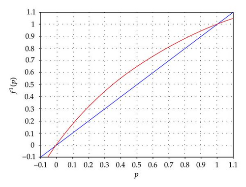
Example 4.1 ((a11 = 10; a12 = 10; a21 = 20; a22 = 20)). The presented classification indicates that, in this case, point p*(1) is unstable and point p*(2) is stable. This is also a case where these are the only two steady-state points. Thus, point p*(2) is globally stable, which means that p converges to 1 and thus strategy D is evolutionarily stable: independently of the initial value of the share p, individuals will tend to adopt this strategy, which becomes the only one that is chosen in the long run. Figure 2 presents the corresponding phase diagram.
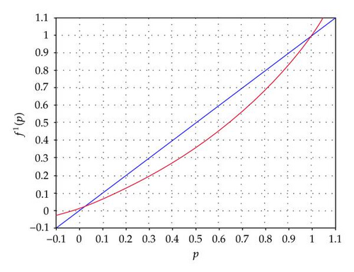
Example 4.2 ((a11 = 20; a12 = 20; a21 = 10; a22 = 10)). Now, we have the opposite situation. Point p*(1) is stable and point p*(2) is unstable. Strategy D is not evolutionarily stable, that is, all the individuals in the population will avoid following this strategy in the long run. Again, these are the only two steady-state values and, accordingly, H must be an ESS. In Figure 3, the phase diagram is displayed.
Example 4.3 ((a11 = 10; a12 = 20; a21 = 20; a22 = 10)). In this setting, both mentioned steady-state points are unstable; thus, there is divergence relatively to a scenario of pure choice of one of the two strategies. However, in this case there is a third steady-state p*(3) = 1/2. Replacing this steady-state value into the derivative expression alongside with the payoff values and the initial fitness, we arrive to ; since this value is inside the unit circle, we confirm the stability of this point. In this type of setting, for any initial p0 value in the interval (0,1), there is a convergence to an outcome according to which in the long-run half of the population will choose one strategy while the other will adopt the alternative strategy. Figure 4 illustrates this case.
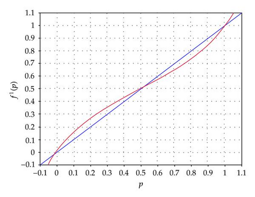
Example 4.4 ((a11 = 20; a12 = 10; a21 = 10; a22 = 20)). The current case is such that both steady-state values p*(1) and p*(2) correspond to points of local stability. Again, an intermediate steady-state value exists, p*(3) = 1/2, but now this is unstable, because is outside the unit circle. The point p* = 1/2 constitutes a borderline for convergence; for an initial value above this point, there is evolutionary stability of strategy D (there is convergence towards full adoption of this strategy); for an initial value below the referred point, strategy D will be evolutionarily unstable (i.e., point p*(1) = 0 is stable and, therefore, no individual will select this strategy in the long term, meaning that H is the ESS). Figure 5 presents the phase diagram in this last example.
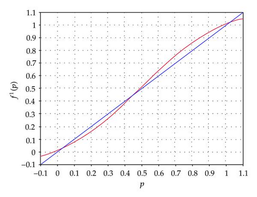
In the above examples, stability holds for one or more than one of the two or three steady-state points that eventually exist. These examples do not involve any specific real life interaction process. In Section 6, we attribute possible meanings to the payoffs and explore cases where none of the steady-state points is stable.
5. Discrete Dynamics and Heterogeneity of Expectations
where is the derivative computed in the previous section for the equation referring to the replicator dynamics.
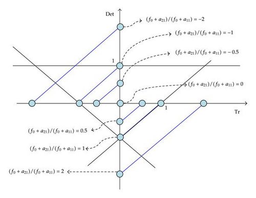
To address the stability of the steady-state points, we must evaluate stability conditions of the two-dimensional system. This requires computing trace and determinant of the Jacobian matrix in the above expression, for each of the steady-state points. Let us concentrate attention in point p*(1). The trace of the corresponding matrix is Tr = ((f0 + a21)/(f0 + a11))x, while the determinant is Det = −((f0 + a21)/(f0 + a11))(1 − x). Figure 6 allows to characterize the stability properties associated to the considered equilibrium point. This figure relates the trace and the determinant expressions. The lines that form the inverted triangle are bifurcation lines; the stability region is precisely the one inside such triangle. For every possible value of x, we can establish the relation Det = Tr − (f0 + a21)/(f0 + a11) and represent it graphically. Note that the constraint x ∈ [0,1] will imply that Tr ∈ [0, (f0 + a21)/(f0 + a11 )] and Det ∈ [−(f0 + a21)/(f0 + a11), 0]. The figure displays straight lines, one for each one of a series of selected values of (f0 + a21)/(f0 + a11). The dynamic results will have some similarities with the results in the one-dimensional replicator dynamics case (which can be understood in this graphic by following the horizontal axis, i.e., by taking the limit case x = 1). For positive and larger than 1 values of (f0 + a21)/(f0 + a11), the dynamics fall outside the stability triangle and for values of (f0 + a21)/(f0 + a11) between −1 and 1, stability will hold (independently of the value of x). The difference between the two cases will occur for values of (f0 + a21)/(f0 + a11) lower than −1; under plain replicator dynamics, the corresponding equilibrium value is locally unstable, while in this second more general setting, stability becomes possible, as long as the specified ratio is not larger than −3. For instance, when (f0 + a21)/(f0 + a11) = −2, stability will hold for values of x between 1/2 and 3/4.
Evaluating stability for each one of these three steady-state values, we verify, as in the initial circumstance, that p*(1) and p*(2) are stable, while p*(3) is locally unstable. The dominant strategy in the long run may either be D or H, depending on the initial distribution of individuals between selected strategies.
Our conclusion is that as long as , the stability results in this second environment are identical to the ones in the simple replicator rule case, and this occurs independently of the value of x. Differences between the two cases will become relevant for . In the next section, some illustrations will clarify this point. Note that in such case x turns out to be of central importance, that is, the values of α, θ, and λ become determinant for the observed dynamic outcome.
6. Illustrations
6.1. Illustration 1: The Hawk-Dove Game
The strategy Hawk (H) generates a benefit b > 0 that is integrally captured when the other agents follow strategy D. However, a confrontation with another hawk implies not only a need to share the referred benefit but there is also a cost c (0 < c < b) of conflict that reduces the original payoff. If an agent chooses to behave as a dove, he/she loses everything when confronted with a hawk and splits benefits without any conflict if he/she interacts with another dove.
The fitness function of hawks is and the fitness function for doves is .
The first derivative is a positive and lower than 1 value, while the second corresponds to an amount that is larger than 1. Thus, point p*(1) is stable and p*(2) is unstable. This allows us to identify an evolutionarily stable strategy, that is the one for which the share of agents selecting to act as doves is zero, or, putting it differently, it is the strategy hawk. In an uncoordinated environment, everyone in the population finds an advantage in ending up by behaving as hawks; there is an evolutionary process that concentrates behavior in strategy hawk.
Now assume the more sophisticated rule. As referred in the previous section, as long as and are both positive values, the stability properties are the same, regardless of the value assumed by the combination of parameters x. Strategy D is evolutionarily unstable and strategy H is evolutionarily stable also in the more general case where expectations are taken into consideration.
6.2. Illustration 2: Some Popular Games
In this subsection, we explore some well known-interaction situations in game theory. Specifically, three models are addressed, namely, the prisoner’s dilemma, matching pennies, and the grab the dollar game. We briefly refer to the structure of the game and to the dynamic outcome both under the replicator dynamics and under the rule involving expectations.
For an initial positive fitness value, f0, there are various long-run possibilities. We can start by distinguishing cases f0 < bm and f0 > bm. For f0 > bm, the fixed-point p*(2) falls outside the unit circle; for f0 < bm, we realize that p*(2) is outside the unit circle for bm ∈ (f0, 2f0) and inside it under condition bm > 2f0. In case f0 < bm, we also observe that f0 < b < B, and thus p*(1) is an unstable point. Under f0 > bm, f0 can be lower than B and larger than b, larger than both or smaller than both. If f0 > B > b, then the expression (f0 − B)/(f0 − b) is positive and larger than 1; if B > b > f0, then (f0 − B)/(f0 − b) is negative but below −1. If B > f0 > b, than we find a value inside the unit circle under condition b < 2f0 − B. We conclude that any of the strategies can be evolutionarily stable, depending on the values of the payoffs; note, as well, that they cannot be simultaneously stable.
When point p*(1) is stable, not to confess is not an evolutionarily stable strategy; it is evolutionarily stable for a stable p*(2). Let us illustrate the game for two different stability outcomes. Begin by taking the following values: f0 = 2, bm = 6, b = 8, B = 10. This is the case for which inequality bm > 2f0 holds and, therefore, point p*(2) is stable, meaning that not confessing is an evolutionarily stable strategy. In this case, , that is, the steady-state for which no individual selects the not confessing strategy is unstable.
The second example will allow for stability of p*(1), that is, not to confess is an evolutionarily unstable strategy, which implies that confessing is certainly evolutionarily stable. Let f0 = 2, bm = 0.5, b = 0.75, B = 3. The evaluation made above indicates that in this case we have stability of p*(1). To confirm this, observe that −0.8.
In the evolutionary prisoner’s dilemma in discrete time, under the replicator rule, to confess and not to confess are both possible evolutionarily stable outcomes. This result does not depend solely on the payoffs but also on the initial fitness value.
To see what modifications the second assumed dynamic evolutionary rule implies, one needs to recover Figure 6 and locate the dynamics in the corresponding trace-determinant relation. We focus on the two displayed examples. In the first example, and . The first of these points falls outside the triangle representing stability and the second point locates inside such triangle, for every possible value of x. Thus, results are qualitatively the same as for the simple replicator dynamics. For the second example, it is true that and . Again, the more sophisticated dynamic rule produces exactly the same stability result as the first one.
Now, three steady states exist: p*(1) = 0, p*(2) = 1 and p*(3) = 1/2. Next, we observe that . For a positive initial fitness, stability holds for both points. Relatively to p*(3), we compute the derivative . Under f0 > 0, this point is unstable. The evolutionary outcome is, then, the following: for any p0 < 1/2, the long-run result implies the stability of p*(1) = 0, that is, strategy T is evolutionarily unstable (and, thus, strategy H is evolutionarily stable); if p0 > 1/2, then the system converges towards p*(2) = 1, which means that strategy T is evolutionarily stable. The evaluation of the computed derivative values in the more sophisticated dynamic scenario will generate precisely the same qualitative dynamic results; to confirm this, we just need to locate the straight lines corresponding to (f0 − 1)/(f0 + 1)∈(−1,1) and (f0 + 1)/f0 > 1 in the diagram of Figure 6.
Repeating the same procedure as in the previous cases, we notice that p*(3) = 1/2 is a viable steady state. The evaluation of local stability yields the following outcomes: , and . Taking f0 > 0, as before, we realize that p*(1) and p*(2) are unstable points, while p*(3) is stable for f0 > 0.25. Under inequality f0 ≤ 0.25, there is no stable steady state. In this case, we will find a bounded instability outcome, with persistent fluctuations in time. Figures 7 and 8 illustrate the case for f0 = 0.18. It is presented a phase diagram and the trajectory of p in time. The phase diagram allows to realize that the chaotic dynamic result is obtained under a given basin of attraction; namely, we must consider p > 0.3595.
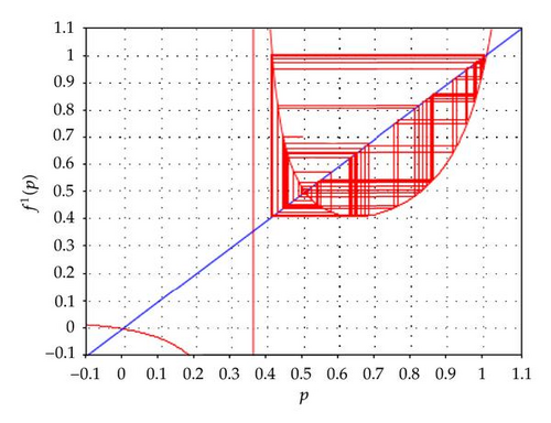
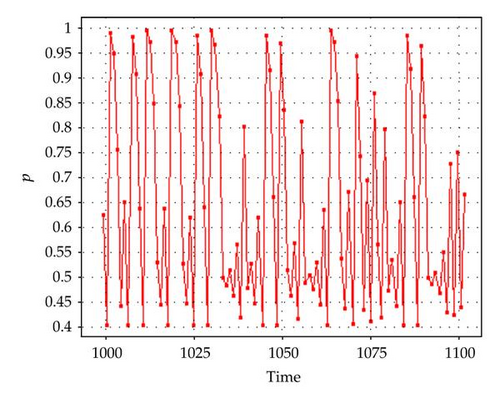
We can characterize the results of this game in the following manner. For a not too low initial fitness (f0 > 0.25), the game generates a result where half of the firms choose to invest and the other half does not invest. For low values of f0, we may have perpetual motion in turn of such equilibrium.
In this simple example, built upon a perfectly logical strategic environment, we find a result where permanent mobility from one strategy to the other exists. Is this result maintained for the second dynamic rule we have considered? For the dynamic rule involving expectations, the two extreme steady states continue to fall in the instability region. The steady-state p*(3) will also continue to represent a stable outcome as long as f0 > 0.25, independently of the value of the combination of parameters x; however, when f0 ≤ 0.25, we fall in the region of Figure 6 where, for intermediate values of x, stability might prevail, although this is not true for levels of x near 0 or 1. Consider again f0 = 0.18; Figure 9 presents a bifurcation diagram where x is the bifurcation parameter. The scenario just described is illustrated; nonlinear dynamics are present for most values of x, excluding a small intermediate region of stability (recall that the replicator dynamics correspond to the setting for which x = 1). In Figure 10, a strange attractor reflecting the presence of chaotic motion is drawn for x = 0.2.
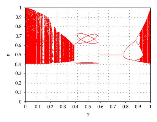
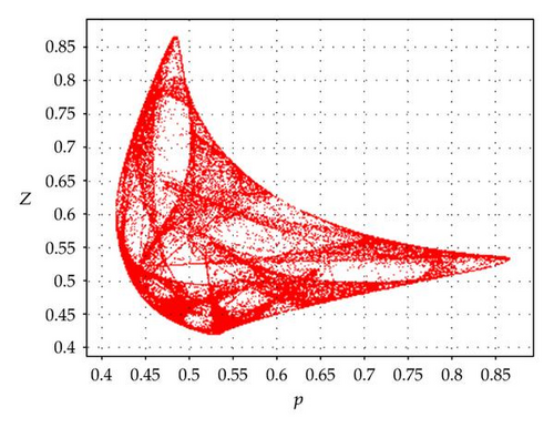
The difference in outcomes between the two alternative dynamic rules is well reflected in this example. As referred when presented the general case, such difference is visible only when the derivative dpt+1/dpt, evaluated in the vicinity of the steady-state point, falls between −3 and −1. This is the single case where it is relevant, in terms of stability results, the value assumed by the combination of parameters x.
6.3. Illustration 3: A Class of Nonlinear Outcomes
Computation of derivatives of the above expression leads to and . Stability will eventually hold solely for p*(3) = a1/(a1 + a2). For this steady-state value, . Stability of p*(3) is guaranteed for . The first inequality is satisfied for and the second requires . It is the violation of this second condition that leads to the occurrence of nonlinear outcomes that exist both for the replicator dynamics and for the lagged dynamic rule.
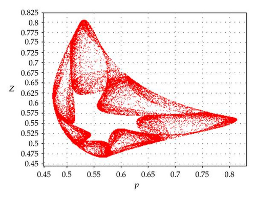
As an example, consider the second dynamic rule and the following parameter values: f0 = 2, a1 = 12, a2 = 10. In this case, and therefore it is feasible the existence of endogenous fluctuations. Figure 11 displays the strange attractor formed, in this case, for x = 0.21.
7. Conclusion
The paper has addressed stability properties of dynamic systems in the context of evolutionary games. In a discrete time context, with only two available strategies for each one of the members of a given population, we have identified multiple possibilities in terms of long-term outcomes, which are dependent on payoffs, initial fitness, and assumed dynamic rule. The richness of the analysis is evidenced by the variety of results that such a simple setting allows to obtain. A given strategy may be evolutionarily stable, in the sense that all the players will end up by following it in the long term, or evolutionarily unstable, case in which the agents prefer to migrate to the alternative strategy. However, there is a third possibility that was also discussed. If none of the strategies qualify as evolutionarily stable, the outcome of the game may be a long-run locus where a share of the individuals in a population sticks with one of the strategies, while the remaining share prefers to follow the alternative strategy. Moreover, it is also conceivable a scenario where this is a floating share that does not converge to a resting point and with a trajectory characterized by regular or irregular cycles.
The dynamic result of a strategic interaction relation is contingent on the type of intertemporal rule that is considered for the evolution of the probability of selecting one or the other strategy. In economics, it makes sense to go beyond a purely evolutionary rule, where the only criterion for changing or maintaining some strategy relies on its past performance. A forward looking behavior must be introduced in the considered dynamic rule. Combining the notions of replication of past results and decision-making based on past expectations, we have suggested a more complete adjustment mechanism. Under this, long-term behavior may deviate from the benchmark case, namely, in scenarios where bifurcations trigger the transition between regions of stability and regions where endogenous fluctuations are observable.
Acknowledgment
The author would like to acknowledge financial support from his research center—the Business Research Unit of the Lisbon University Institute—under project number PEst-OE/EGE/UI0315/2011, without which it would not have beeen possible to publish this work.


