On the Solution of a Class of Nonlinear Systems Governed by an M-Matrix
Abstract
We consider a weakly nonlinear system of the form (I + φ(x)A)x = p, where φ(x) is a real function of the unknown vector x, and (I + φ(x)A) is an M-matrix. We propose to solve it by means of a sequence of linear systems defined by the iteration procedure (I + φ(xr)A)xr+1 = p, r = 0, 1, …. The global convergence is proved by considering a related fixed-point problem.
1. Introduction
- (i)
p ∈ RN with p > 0;
- (ii)
A ∈ RN×N has nonnegative main diagonal and nonpositive off-diagonal entries (Z-matrix);
- (iii)
A is rowwise weakly diagonal dominant;
- (iv)
φ : RN → R is a differentiable function such that φ(x) ≥ 0, for all x ≥ 0 and it is homogeneous of degree γ ≤ 1, that is, for all α > 0 φ(αx) = αγφ(x);
- (v)
grad(φ(x)) > 0 for all x ≥ 0, where grad(φ(x)) denotes the (row vector) gradient of φ(x).
A central rule in our results is played by the matrix (I + φ(x)A) appearing in (1.2) which, as it can be immediately seen from the assumption (ii)‒(iv), is an M-matrix for all x ≥ 0 (see, e.g., [5, page 137, prop. M35]).
The organization of the paper is the following. In Section 2, we investigate a particular class of one variable functions f such that the FP iterations tr+1 = f(tr) converge independently of the choice of the starting value t0. By exploiting this result jointly with the properties of the matrix I + φ(x)A, we are lead to state that, under the assumptions (i)–(v), the FP iteration procedure (I + φ(xr)A)xr+1 = p globally converges to a solution of (1.2). This constitutes our main result which is contained in Section 3. Finally, some numerical experiments showing the sharpness of the required conditions and the performance of the iteration scheme are reported in Section 4.
2. The One Variable Case
In order to prove our main theorem, we need the following result on a particular class of numerical sequences.
Theorem 2.1. Let f be a one variable scalar function such that
- (a)
f : t ∈ X⊆[0, +∞)→(0, Mf), with Mf > 0, X closed and f(X) ⊂ X;
- (b)
f continuous;
- (c)
tf(t) strictly increasing.
In this section, we are going to prove this theorem.
Lemma 2.2. If g(tr) < 0 (resp. > 0) and g(tr+m) > 0 (resp. < 0), m = 1, …, n, then
Proof. Let us prove (2.4) by induction on n ≥ 1. Assume n = 1, that is, we are assuming that
Now, we assume that the lemma holds for m = n, that is, suppose that
In order to state Theorem 2.1, we are going to prove that these subsequences converge to the same limit. First of all, the following result holds.
Lemma 2.3. The sequences and are strictly increasing and decreasing respectively.
Proof. Let us prove that the sequence is strictly increasing, the proof about is analogous, and it is omitted. Consider ri such that . Then, two cases may occur: (I) or (II) .
- (I)
In this case, it is clear that belongs to the same subsequence and we immediately have
(2.20) - (II)
From (2.3), there exists n ≥ 2 such that , that is, we have
Lemma 2.4. The sequences and provide two separate sets, that is,
Proof. Suppose, for example, ri < sj and precisely let sj = ri + k. If k = 1, we get (2.24) directly from the assumption . If k ≥ 2, observe that the numerical sequence presents at least one change of sign, in view of (2.19). Let us examine the case of an unique change of sign, by supposing that there exists an integer l, with 0 ≤ l ≤ k − 1, such that
By Lemma 2.3, we get
By the previous lemmas, we get the next result which completes the proof of the convergence of the FP iteration process.
Theorem 2.5. For any choice of t0 ∈ X, the sequence {tr} r defined in (2.1) converges.
Proof. It is sufficient to prove that the subsequences and defined in (2.19) converge to the same limit, satisfying
3. The Solution of the Nonlinear System
Theorem 3.1. Assume that (i)–(v) hold. Then, F is a continuous, differentiable function, and for any q ≥ 0, it satisfies
Proof. As the inverse of (I + qA) is defined for all q ≥ 0, then F is clearly a continuous function. Moreover, it can be easily seen that
Using this theorem, we can easily claim that the function F in (3.2) has the same characteristics as the function f introduced in the previous section.
Corollary 3.2. Assume that (i)–(v) hold. Then, the function F verifies all the hypotheses (a)–(c).
Proof. Assertions (a) and (b) directly follow from Theorem 3.1. Moreover, in view of (3.5), (c) is immediately obtained by qF(q) = s(q)q1−γ, recalling that γ < 1 implies q1−γ strictly increasing.
Theorem 3.3. Assume that the hypotheses (i)–(v) hold. Then, the sequence {xr} converges to a solution x* of (1.2).
Proof. Let us start from an arbitrary x0 ≥ 0 and put
Remark 3.4. Of course, in view of (3.7), any solution of (1.2) satisfies ∥x*∥∞ ≤ ∥p∥∞, but nothing seems to imply its uniqueness. Anyway, we conjecture it, because in a large variety of experimental tests (including also high-dimensional systems), we never found more than one solution. Of course, a sufficient condition for the uniqueness is ∥grad(φ(x))∥1∥A∥∞∥p∥∞ < 1, for any x ≥ 0, which assures |F′(q)| < 1, for any q ≥ 0, by virtue of (3.4) and (3.7). Nevertheless, as it can be observed in the next section, it seems that the solution is unique even if such a condition is largely not satisfied.
4. Numerical Experiments
| FP iterations. | 15 | 14 | 14 | 15 |
|---|---|---|---|---|
| q0 | .2 | .4 | 1 | 100 |
| fzero iterations. | 21 + 4 | 19 + 4 | 16 + 4 | 12 + 6 |
| FP iterations. | 19 | 19 | 19 | 17 | 20 |
|---|---|---|---|---|---|
| q0 | .05 | .1 | 1 | 2 | 100 |
| fzero iterations. | AB | AB | AB | 11 | AB |
| FP + fzero iterations. | 1 + 13 | 1 + 15 | 1 + 12 | 3 + 4 | 2 + 13 |
From these two tests, we observe that, according to Theorem 3.3, the FP iteration method converges for any q0 in both the cases. Of course, when we know the interval where a zero lies, fzero does converge and it requires much less iterations, but in many cases this information is unavailable and, see Table 2, fzero fails to provide a value. In fact, at the third line of Table 2, the symbol AB stays for “aborted” and means that the MATLAB routine does not succeed in finding an interval containing a sign change. The last line of Table 2 shows that the best results can be obtained by a combined solution strategy, which starts with a certain number of FP iterations (first addendum) and takes the final steps using fzero iterations (second addendum). At the fifth column, we take the right balance between FP and fzero iterations, while in the remaining columns, we displayed the minimum number of FP iterations which are necessary to get a value from fzero. Thus, we can fruitfully exploit the global convergence of our FP iteration method in order to create more efficient combined strategy with fzero. Of course, this could be done also by means of other well-known methods like Newton’s one.
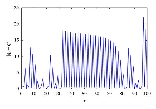
In order to verify whether the convergence of the FP procedure could be ascribed to the Banach contraction theorem, we plotted the absolute value of the derivative of the function F in (4.1) (not reported) and we noted that the starting value in bold, that is, q0 = .2, q0 = .4 in Table 1 and q0 = .05, q0 = .1 in Table 2, belongs to intervals where |F′(q)| > 1. Hence we can assert that, at least in these cases, the convergence of the FP method is not “helped” by the contraction principle.
As we already wrote in Remark 3.4, from these numerical experiments and many others, starting from very different values of q0, the method seems to converge to the same fixed point. For example, in problems (4.2) and (4.3), we obtain q* ≈ 4.7954 and q* ≈ 2.6085, respectively, for a very large number of initial guesses (much larger than the ones reported in Tables 1 and 2). This numerical evidence let us conjecture that the assumptions in Theorem 3.3 are also sufficient to assure the uniqueness of the solution of problem (1.2).


Moreover, we point out that, in our experience, some problems arising in the the kinetic theory of dusty plasmas, are more cumbersome than (1.1), and therefore, the application of Newton or other available iterative procedures is not always simple, convenient, or possible. A comparison between FP and other iteration processes on problem of type (1.1) will be the subject of future investigations. Finally, in order to test the performance of our method for larger systems arising from the applications, we discretized a problem of type (1.1) with stepsize h on a sufficiently large interval (0, T), with T = Nh. In this way, we get a nonlinear system of type (1.2), which has dimension N. By applying FP iteration method to such a system for different values of N, with 102 < N < 105, we observe that the number of iterations does not vary with N and so with h, but only with the choice of the starting point q0. Moreover, we underline that in this case the linear systems arising from the FP iterations are tridiagonal and then very easy to be solved.


