Volume 2012, Issue 1 370894

Research Article

Open Access

Fixed-Point Iterative Algorithm for the Linear Fredholm-Volterra Integro-Differential Equation

Corresponding Author

M. I. Berenguer

[email protected]

Departamento de Matemática Aplicada, E.T.S. de Ingeniería de Edificación, Universidad de Granada, 18071 Granada, Spain ugr.es

Search for more papers by this author

D. Gámez,

D. Gámez

Departamento de Matemática Aplicada, E.T.S. de Ingeniería de Edificación, Universidad de Granada, 18071 Granada, Spain ugr.es

Search for more papers by this author

A. J. López Linares,

A. J. López Linares

Departamento de Matemática Aplicada, E.T.S. de Ingeniería de Edificación, Universidad de Granada, 18071 Granada, Spain ugr.es

Search for more papers by this author

M. I. Berenguer,

Corresponding Author

M. I. Berenguer

[email protected]

Departamento de Matemática Aplicada, E.T.S. de Ingeniería de Edificación, Universidad de Granada, 18071 Granada, Spain ugr.es

Search for more papers by this author

D. Gámez,

D. Gámez

Departamento de Matemática Aplicada, E.T.S. de Ingeniería de Edificación, Universidad de Granada, 18071 Granada, Spain ugr.es

Search for more papers by this author

A. J. López Linares,

A. J. López Linares

Departamento de Matemática Aplicada, E.T.S. de Ingeniería de Edificación, Universidad de Granada, 18071 Granada, Spain ugr.es

Search for more papers by this author

First published: 08 July 2012

https://doi.org/10.1155/2012/370894

Citations: 6

Academic Editor: Rudong Chen

Share a link

Email
Wechat
Bluesky

Abstract

With the aid of fixed-point theorem (an equivalent version for the linear case) and biorthogonal systems in adequate Banach spaces, the problem of approximating the solution of a linear Fredholm-Volterra integro-differential equation is turned into a numerical algorithm, so that it can be solved numerically.

1. Introduction

Denoting by 𝒞([0,1]) and 𝒞([0,1] ²) the Banach space of all continuous and real-valued functions defined on [0,1] and [0,1] ², respectively, equipped with their usual sup-sup norm, let us consider the following problem associated to the Fredholm-Volterra integro-differential equation: given ρ ∈ ℝ, k₁, k₂ ∈ 𝒞([0,1] ²), and f, x₀ ∈ 𝒞([0,1]), find x ∈ 𝒞¹([0,1]) such that

()

Observe that if k₁(t, s) = 0 and f(t) = 0 in (1.1), the equation is transformed into a linear Volterra integro-differential equation; and if k₂(t, s) = 0 and f(t) = 0, it becomes a linear Fredholm integro-differential. Additionally, if k₁(t, s) = k₂(t, s) = 0, (1.1) is transformed into a linear differential equation of the first order.

Frequently the mathematical modelling of problems arising from the real world (see [1] and the references therein) deals with problem (1.1). These are usually difficult to solve analytically, and in many cases, the solution must be approximated. Therefore, in recent years, several numerical approaches have been proposed (see, e.g., [2–4]). The numerical methods usually transform the integro-differential equation into a linear system that can be solved by direct or iterative methods. On the other hand, the use of fixed-point techniques in the numerical study of linear differential, integral, and integro-differential equations has also proven successful in some works, as [5–11]. The purpose of this paper is to develop an effective method for approximating the solution of (1.1) using Schauder basis and another classical tool in analysis: an equivalent version of the fixed-point theorem for the linear case (the geometric series theorem). This algorithm generalizes the developed ones in [7, 8, 10] for Volterra integro-differential, Fredholm integro-differential, and differential equation, respectively.

To establish our numerical method, we first need to review some results of a theoretical nature in Section 2. We arrive at a numerical method for approximating the solution of (1.1) in Section 3, and in order to state the results about convergence and to study the error of the proposed algorithm, we will assume that γ = ∥f∥+∥k₁∥+∥k₂∥/2 < 1 and k₁, k₂ ∈ C¹([0,1] ²) and f, g ∈ C¹([0,1]). Finally, in Section 4, we illustrate the theoretical results with two examples.

2. Two Tools of a Theoretical Nature

Two fundamental tools will be used to establish the algorithm needed to solve the problem (1.1). The first is the following equivalent version (for the linear case) of the Banach fixed-point theorem (see [12]).

Geometric Series Theorem Let X be a Banach space, and let T : X → X be a continuous and linear operator such that ∥T∥<1. Then, Id − T is a continuous, linear, and bijective operator and (Id − T) ⁻¹ = ∑_n≥0 Tⁿ.

In particular, given y ∈ X, the equation (Id − T)x = y has a unique solution x = (Id − T) ⁻¹y.

The second tool applied consists of biorthogonal systems in Banach spaces 𝒞([0,1]) and 𝒞([0,1] ²). We will make use of the usual Schauder basis for simplicity in the exposition, although the numerical method given works equally well by replacing it with any complete biorthogonal system in 𝒞([0,1] ²). For this reason, we will now briefly recall the main issues and notations regarding Schauder bases in 𝒞([0,1]) and 𝒞([0,1] ²).

Let us consider the usual Schauder basis {b_n} _n≥1 in the space 𝒞([0,1]), that is, for a dense sequence

of distinct real numbers in [0,1] such that t₁ = 0 and t₂ = 1, we define b₁(t): = 1 for t ∈ [0,1], and for n ≥ 2, b_n is the piecewise linear continuous function on [0,1] with nodes at {t_i : 1 ≤ i ≤ n}, uniquely determined by the relations b_n(t_n) = 1 and b_n(t_k) = 0 for k < n. For each function z ∈ 𝒞([0,1]), there exists a unique sequence of scalars

such that z = ∑_n≥1 β_nb_n. We denote by

the sequence of (continuous and linear) biorthogonal functionals in the dual space of 𝒞([0,1]), defined by

()

whereas the sequence of (continuous and linear) projections

is defined by the partial sums

()

For the respective sequence of biorthogonal systems

and each z ∈ 𝒞([0,1]), the equalities

()

are valid (see [13]). As a consequence, the sequence of associated projections

satisfies the following interpolation property:

()

We now evoke the construction of the usual Schauder basis

for the Banach space 𝒞([0,1] ²), endowed with its usual sup-norm (see [13, 14]). To this end, we consider the bijective mapping τ : ℕ → ℕ × ℕ (where [p] denotes the integer part of p) given by

()

Then it suffices to define

()

whenever τ(n) = (i, j). Let

and

stand for the corresponding sequences of biorthogonal functionals and projections, respectively. The Schauder basis

has similar properties to those of the one-dimensional basis

(a)
for all t, s ∈ [0,1], B₁(t, s) = 1 and for n ≥ 2,
(b)
if w ∈ C([0,1] ²), then , and for all n ≥ 2, if τ(n) = (i, j), ,
(c)
the sequence of associated projections satisfies Q_n(w)(t_i, t_j) = w(t_i, t_j), whenever n, i, j ∈ ℕ and τ⁻¹(i, j) ≤ n,
(d)
this Schauder basis is monotone, that is,

Observe that for each n ∈ ℕ, the definition of the projections P_n and

requires only the first n + 1 points of the sequence

. These n + 1 points, sorted in increasing order, constitute a partition of the interval [0,1], which will be denoted as T_n; let ΔT_n denote the maximum distance between two consecutive points of T_n. Under some weak conditions, from (2.4) and (c), respectively, and the mean-value theorem, we can estimate the rate of convergence of the sequence of projections:

()

3. The Algorithm: Convergence and Error

Our starting point is the formulation of (1.1) in terms of a certain operator L as follows: let L : 𝒞([0,1]) → 𝒞([0,1]) be the linear and continuous operator defined by

()

It is a simple matter to check that a function x ∈ C¹([0,1]) is the solution of (1.1) if and only if (Id − L)x = g, where .

It can be shown by an induction argument and Fubini′s theorem that for j ∈ ℕ, ∥L^jx∥≤∥x∥γ^j; hence,

()

The condition assumed on γ and the geometric series theorem allow us to establish the existence of one and only one solution x of (1.1), which is

()

Besides,

()

In view of (3.3), we consider the sequence

defined as follows: y₀(t) = L⁰g(t) = g(t), and for m ≥ 1,

()

The sequence

converges to the solution x of (1.1) and

()

We can then calculate iteratively using (3.5), at least in a theoretical way, the solution of (1.1). From a practical viewpoint, in general these calculations are not possible explicitly. The idea of our numerical method is to use an appropriate Schauder basis in the spaces 𝒞([0,1]), 𝒞([0,1] ²) truncating the functions of such spaces by means of the projections of the Schauder bases and , and replacing each Ly_m−1 (m ≥ 1) in (3.5) by a new function v_m ∈ 𝒞([0,1]), easier to calculate, and in such a way that the error ∥x − (g + v_m)∥ be small enough. Given these functions, each g + v_m will be approximation of the solution of (1.1).

Specifically, we begin with v₀(t) = 0 and consider

()

Letting m ∈ ℕ, we inductively define the functions

()

where n_m are natural numbers.

We will show that the sequence approximates the solution of (1.1) while in order to study the error , let us assume that k₁, k₂ ∈ C¹([0,1] ²) and f, g ∈ C¹([0,1]).

In the first place, we show the following.

Lemma 3.1. The sequences and are bounded.

Proof. First we show, using an inductive argument, that for all t ∈ [0,1], . Since the Schauder basis is monotone, we have

()

Suppose that the result holds for m − 1, in other words , and using the monotony of , we prove for m the following:

()

Therefore, ∥v_m∥≤∥g∥∑_j≥1 γ^j.

On the other hand, with similar arguments,

()

and thus,

Remark 3.2. Given that for i ∈ {1,2} and m ∈ ℕ,

()

denoting by

()

we have that the sequence

is also bounded.

Theorem 3.3. With the previous notation, if m ∈ ℕ, with n_j+1 ≥ 2 and M = sup {M_m} _m∈ℕ, then

()

Proof. The triangle inequality gives . Because of the inequality (3.6), we have

()

For the second one, by an inductive argument, we can show that

()

Indeed, for m = 1, the result is clearly true

()

Suppose it holds for m − 1, that is,

, and we prove for m the following:

()

Then

()

For j = 0,1, …, m − 1,

()

And thus, applying (2.7), we obtain the following bound:

()

The proof is complete in view of the triangular inequality and of (3.6) and (3.16).

Remark 3.4 3.4. Under the hypothesis of Theorem 3.3, for all ε > 0, we can find m ∈ ℕ and positive integers n₁, …, n_m such that . Furthermore, since γ < 1 and the points of partition can be chosen such that h is as small as we desire, is as small as we desire, and (3.14) also provides a quota of the error committed when we approach x by .

Remark 3.5. It follows from Theorem 3.3 that the proposed method with the chosen Schauder bases has order of convergence one. This choice has been done by simplicity in the exhibition of the results, and it has allowed us to obtain satisfactory numerical results as we show in the following section. Nevertheless, by integrating the considered basis in 𝒞([0,1]) (and adding the one constant function), we obtain new bases of 𝒞([0,1]) and 𝒞([0,1] ²). Considering these bases, the order of convergence is 2. In general, integrating n + 1 times, we would obtain order of convergence n.

4. Some Numerical Example

We now turn our attention to show two numerical performance results. For each example, we have fixed the subset chosen for constructing the Schauder basis in 𝒞([0,1]) and in 𝒞([0,1] ²), specifically, t₁ = 0, t₂ = 1; and for n ∈ ℕ ∪ {0}, t_i+1 = (2k + 1)/2ⁿ⁺¹ if i = 2ⁿ + k + 1 where 0 ≤ k < 2ⁿ are integers. To define the sequence , we take n_j = i (for all j ≥ 1). In addition we include, a table exhibiting, for i = 9,17, and 33, the absolute errors committed for certain representative points of [0,1] when we approximate the exact solution x(t) by means of the iteration where m is shown in the table. The algorithms associated with the numerical method were performed using Mathematica 7. We have checked that when more points are used, the accuracy improves significantly, unlike the number of iterations.

In order to provide some details, we synthesize the steps of the programmed algorithm:

(1)
we introduce the nodes; we construct the base {b_n} and the base {B_n},
(2)
we calculate g (if it is not possible to explicitly arrive at g, we can apply a quadrature method),
(3)
we define v₀(t) = 0 and ,
(4)
we calculate and using the base {b_n} and , , , and using the base {B_n}. Note that we calculate the projections by integrals of piecewise univariate and bivariate polynomials of degrees 1 and 2 and the calculation of the coefficients of such polynomials just requires linear combinations of several evaluations of the basic functions at adequate points. We do not have to solve systems of algebraic equations,
(5)
we calculate the expression using Definition (3.8),
(6)
repeat the process.

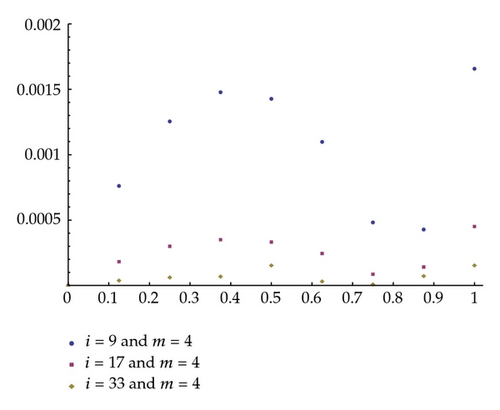
Example 4.1. For the first example, we consider the following linear Fredholm-Volterra integro-differential equation with the exact solution x(t) = t². Its numerical results are given in Table 1 and Figure 1:

()

Table 1. Absolute errors for Example 4.1.

t	i = 9	i = 17	i = 33
t
0.125	7.63E − 4	1.84E − 4	4.04E − 5
0.250	1.25E − 3	3.02E − 4	6.42E − 5
0.375	1.47E − 3	3.52E − 4	7.12E − 5
0.5	1.42E − 3	3.35E − 4	6.11E − 5
0.625	1.10E − 3	2.47E − 4	3.36E − 5
0.750	4.84E − 4	8.88E − 5	1.15E − 5
0.875	4.30E − 4	1.44E − 4	7.47E − 5
1	1.65E − 3	4.54E − 4	1.56E − 4

Details are in the caption following the image — **Figure 1**
Open in figure viewer PowerPoint

The plot of absolute errors by our method for Example 4.1.

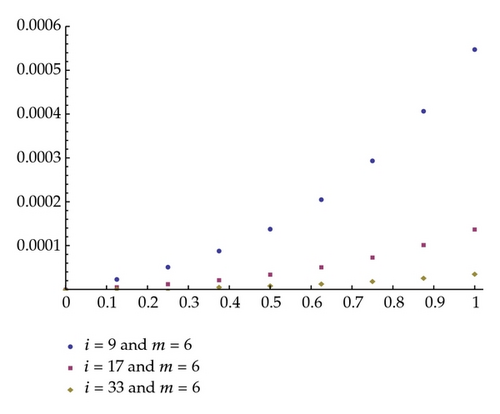
Example 4.2. For the second example, we consider the following linear Fredholm-Volterra integro-differential equation with the exact solution x(t) = t. Its numerical results are given in Table 2 and Figure 2:

()

Table 2. Absolute errors for Example 4.2.

t	i = 9	i = 17	i = 33
t
0.125	2.35E − 5	5.90E − 6	1.51E − 6
0.250	5.15E − 5	1.29E − 5	3.32E − 6
0.375	8.83E − 5	2.21E − 5	5.68E − 6
0.5	1.38E − 4	3.46E − 5	8.90E − 6
0.625	2.05E − 4	5.15E − 5	1.32E − 5
0.750	2.94E − 4	7.37E − 5	1.89E − 5
0.875	4.07E − 4	1.02E − 4	2.63E − 5
1	5.48E − 4	1.37E − 4	3.56E − 5

5. Conclusions

An efficient approach easy to implement is proposed to solve the linear Fredholm-Volterra integro-differential equations. The approximating functions are the sum of integrals of piecewise bivariate polynomials of degree 2, and the calculation of the coefficients of such polynomials just requires linear combinations of several evaluations of the basic functions at adequate points. The approach leads to an approximate solution of the integro-differential equation, which can be expressed explicitly in simple closed form, and which can be effectively computed using symbolic computing codes on any personal computer.

Acknowledgments

This research is partially supported by Junta de Andalucía Grant FQM359 and the ETSIE of the University of Granada.

References

1 Rahman M., Jackiewicz Z., and Welfert B. D., Stochastic approximations of perturbed Fredholm Volterra integro-differential equation arising in mathematical neurosciences, Applied Mathematics and Computation. (2007) 186, no. 2, 1173–1182, https://doi.org/10.1016/j.amc.2006.07.137, 2316739, ZBL1117.65014.
10.1016/j.amc.2006.07.137
Web of Science® Google Scholar
2 Huang Y. and Li X.-F., Approximate solution of a class of linear integro-differential equations by Taylor expansion method, International Journal of Computer Mathematics. (2010) 87, no. 6, 1277–1288, https://doi.org/10.1080/00207160802275969, 2665728, ZBL1191.65179.
10.1080/00207160802275969
Web of Science® Google Scholar
3 Maleknejad K., Basirat B., and Hashemizadeh E., A Berstein operational matrix approach for solving a system of high order linear Volterra-Fredholm integro-differential equations, Mathematical and Computer Modelling. (2012) 55, 1363–1372.
10.1016/j.mcm.2011.10.015
Google Scholar
4 Yalçınbaş S. and Sezer M., The approximate solution of high-order linear Volterra-Fredholm integro-differential equations in terms of Taylor polynomials, Applied Mathematics and Computation. (2000) 112, no. 2-3, 291–308, https://doi.org/10.1016/S0096%2D3003(99)00059%2D4, 1758715, ZBL1023.65147.
10.1016/S0096-3003(99)00059-4
Web of Science® Google Scholar
5 Berenguer M. I., Garralda-Guillem A. I., and Ruiz Galán M., An approximation method for solving systems of Volterra integro-differential equations, Applied Numerical Mathematics. In presshttps://doi.org/10.1016/j.apnum.2011.03.007.
10.1016/j.apnum.2011.03.007
Google Scholar
6 Berenguer M. I., Gámez D., Garralda-Guillem A. I., Ruiz Galán M., and Serrano Pérez M. C., Analytical techniques for a numerical solution of the linear Volterra integral equation of the second kind, Abstract and Applied Analysis. (2009) 2009, 12, 149367, https://doi.org/10.1155/2009/149367, 2564002, ZBL1187.65140.
10.1155/2009/149367
Google Scholar
7 Berenguer M. I., Fortes M. A., Garralda Guillem A. I., and Ruiz Galán M., Linear Volterra integro-differential equation and Schauder bases, Applied Mathematics and Computation. (2004) 159, no. 2, 495–507, https://doi.org/10.1016/j.amc.2003.08.132, 2096721, ZBL1068.65143.
10.1016/j.amc.2003.08.132
Web of Science® Google Scholar
8 Berenguer M. I., Fernández Muñoz M. V., Garralda-Guillem A. I., and Ruiz Galán M., A sequential approach for solving the Fredholm integro-differential equation, Applied Numerical Mathematics. (2012) 62, 297–304.
10.1016/j.apnum.2011.03.009
Web of Science® Google Scholar
9 Caliò F., Fernández Muñoz M. V., and Marchetti E., Direct and iterative methods for the numerical solution of mixed integral equations, Applied Mathematics and Computation. (2010) 216, no. 12, 3739–3746, https://doi.org/10.1016/j.amc.2010.05.032, 2661738, ZBL1195.65223.
10.1016/j.amc.2010.05.032
Web of Science® Google Scholar
10 Castro E., Gámez D., Garralda Guillem A. I., and Ruiz Galán M., High order linear initialvalue problems and Schauder bases, Applied Mathematical Modelling. (2007) 31, 2629–2638.
10.1016/j.apm.2006.10.013
Web of Science® Google Scholar
11 Palomares A. and Galán M. R., Isomorphisms, Schauder bases in Banach spaces, and numerical solution of integral and differential equations, Numerical Functional Analysis and Optimization. (2005) 26, no. 1, 129–137, https://doi.org/10.1081/NFA%2D200051625, 2128748, ZBL1079.65067.
10.1081/NFA-200051625
Web of Science® Google Scholar
12 Atkinson K. and Han W., Theoretical Numerical Analysis, 2005, 39, 2nd edition, Springer, New York, NY, USA, https://doi.org/10.1007/978%2D0%2D387%2D28769%2D0, 2153422, ZBL1211.74196.
10.1007/978-0-387-28769-0
Google Scholar
13 Semadeni Z., Product Schauder bases and approximation with nodes in spaces of continuous functions, Bulletin de l′Académie Polonaise des Sciences. (1963) 11, 387–391, 0154110, ZBL0124.31703.
Google Scholar
14 Gelbaum B. R. and Gil de Lamadrid J., Bases of tensor products of Banach spaces, Pacific Journal of Mathematics. (1961) 11, 1281–1286, 0147881, ZBL0106.08604.
10.2140/pjm.1961.11.1281
Google Scholar

Citing Literature

All articles

Fixed-Point Iterative Algorithm for the Linear Fredholm-Volterra Integro-Differential Equation

Abstract

1. Introduction

2. Two Tools of a Theoretical Nature

3. The Algorithm: Convergence and Error

4. Some Numerical Example

5. Conclusions

Acknowledgments

References

Citing Literature

Figures

References

Information

About Wiley Online Library

Help & Support

Opportunities

Connect with Wiley

Fixed-Point Iterative Algorithm for the Linear Fredholm-Volterra Integro-Differential Equation

Abstract

1. Introduction

2. Two Tools of a Theoretical Nature

3. The Algorithm: Convergence and Error

4. Some Numerical Example

5. Conclusions

Acknowledgments

References

Citing Literature

Figures

References

Related

Information