An Interactive Procedure to Solve Multi-Objective Decision-Making Problem: An Improvment to STEM Method
Abstract
Decisions in the real-world contexts are often made in the presence of multiple, conflicting, and incommensurate criteria. Multiobjective programming methods such as multiple objective linear programming (MOLP) are techniques used to solve such multiple-criteria decision-making (MCDM) problems. One of the first interactive procedures to solve MOLP is STEM method. In this paper we try to improve STEM method in a way that we search a point in reduced feasible region whose criterion vector is closest to positive ideal criterion vector and furthest to negative ideal criterion vector. Therefore the presented method tries to increase the rate of satisfactoriness of the obtained solution. Finally, a numerical example for illustration of the new method is given to clarify the main results developed in this paper.
1. Introduction
Managerial problems are seldom evaluated with a single or simple goal like profit maximization. Today’s management systems are much more complex, and managers want to attain simultaneous goals, in which some of them conflict. In the other words, decisions in the real-world contexts are often made in the presence of multiple, conflicting, and incommensurate criteria. Particularly, many decision problems at tactical and strategic levels, such as strategic planning problems, have to consider explicitly the models that involve multiple conflicting objectives or attributes.
- (i)
Multiple criteria: each problem has multiple criteria, which can be objectives or attributes.
- (ii)
Conflicting among criteria: multiple criteria conflict with each other.
- (iii)
Incommensurable unit: criteria may have different units of measurement.
- (iv)
Design/selection: solutions to an MCDM problem are either to design the best alternative(s) or to select the best one among previously specified finite alternatives.
- (i)
Multiobjective decision making (MODM).
- (ii)
Multiattribute decision making (MADM).
The main difference between MODM and MADM is that the former concentrates on continuous decision spaces, primarily on mathematical programming with several objective functions, and the latter focuses on problems with discrete decision spaces.
For the further discussion about MODM and MADM, some basic solution concepts and terminologies are supplied by Hwang and Masud [2] and Hwang and Yoon [1].
Criteria are the standard of judgment or rules to test acceptability. In the MCDM literature, it indicates attributes and/or objectives. In this sense, any MCDM problem means either MODM or MADM, but is more used for MADM.
Objectives are the reflections of the desire of decision makers and indicate the direction in which decision makers want to work. An MODM problem, as a result, involves the design of alternatives that optimises or most satisfies the objectives of decision makers.
Goals are things desired by decision makers expressed in terms of a specific state in space and time. Thus, while objectives give the desired direction, goals give a desired (or target) level to achieve.
Attributes are the characteristics, qualities, or performance parameters of alternatives. An MADM problem involves the selection of the best alternative from a pool of preselected alternatives described in terms of their attributes.
We also need to discuss the term alternatives in detail. How to generate alternatives is a significant part of the process of MODM and MADM model building. In almost MODM models, the alternatives can be generated automatically by the models. In most MADM situations, however, it is necessary to generate alternatives manually. Multiobjective programming method such as multiple objective linear programming (MOLP) are techniques used to solve such multiple-criteria decision-making (MCDM) problems.
The future of multiple-objective programming is in its interactive application. In interactive procedures, we conduct an exploration over the region of feasible alternatives for an optimal or satisfactory near-optimal solution. Interactive procedures are characterized by phases of decision making alternating with phases of computation. At each iteration, a solution, or group of solutions, is generated for examination. As a result of examination, the decision maker inputs information to the solution procedure. One of the first interactive procedures to solve MOLP is STEM method.
In this paper we try to improve STEM method in a way that we search a point in reduced feasible region whose criterion vector is closest to positive ideal criterion vector and furthest to negative ideal criterion vector. Therefore the presented method tries to increase the rate of satisfactoriness of the obtained solution.
- (i)
MODM Problems,
- (ii)
Basic definitions,
- (iii)
STEM Method.
In Section 3, we will focus on the proposed method. In Section 4, a numerical example is demonstrated. In Section 5 some conclusions are drawn for the study.
2. Preliminaries
In this section we express the following useful concepts that are taken from [4].
2.1. MODM Problems
Multiobjective decision making is known as the continuous type of the MCDM. The main characteristics of MODM problems are that decision makers need to achieve multiple objectives while these multiple objectives are noncommensurable and conflict with each other.
Example 2.1 (instance of MODM problem). For a profit-making company, in addition to earning money, it also wants to develop new products, provide job security to its employees, and serve the community. Managers want to satisfy the shareholders and, at the same time, enjoy high salaries and expense accounts; employees want to increase their take-home pay and benefits. When a decision is to be made, say, about an investment project, some of these goals complement each other while others conflict.
2.2. Basic Definitions
We have the following notion for a complete optimal solution (for more details, see [5]).
Definition 2.2 (satisfactory solution). A satisfactory solution is a reduced subset of the feasible set that exceeds all of the aspiration levels of each attribute. A set of satisfactory solutions is composed of acceptable alternatives. Satisfactory solutions do not need to be nondominated.
Definition 2.3 (preferred solution). A preferred solution is a nondominated solution selected as the final choice through decision maker’s involvement in the information processing.
In the presented method (and in traditional STEM method), in order to measure the distance between two vectors we use the following metric.
Definition 2.4. Consider the weight vector θ where and θi ≥ 0. These weights define the weighted Tchebychev metric.
2.3. STEM Method
The STEM method [3] is based on minimizing the Tchebychev distance from the ideal point to the criterion space. The parameters of the distance formula and the feasible space can be changed by a normalized weighting method based on the DM’s preferences in the previous solution. The procedure of STEM allows the DM to recognize good solutions and the relative importance of the objectives.
At each iteration, the DM is able to improve some objectives, by sacrificing others. In addition, the DM must provide the maximum amount by which the objective functions can be sacrificed, although it is not necessary to provide tradeoffs on objectives. To carry out an iteration in the STEM method, given a solution x(h−1), the DMs must provide their preferences for objective functions to be improved {fi, i ∈ {1, …, s} − J(h)}, as well as the objective functions to be relaxed fi, i ∈ J(h) with corresponding maximal amounts to relax .
3. Improved STEM Method
The procedure for improving STEM method has been given in the following steps.
Step 1 (construct the first pay-off table). In this step we first maximize each objective function and construct a pay-off table to obtain the positive ideal criterion vector f+ ∈ ℝk.
Let , be the solutions of the following k problems, namely, positive ideal solution:
| f1 | f2 | ⋯ | fk | |
|---|---|---|---|---|
| f1 | f12 | ⋯ | f1k | |
| f2 | f21 | ⋯ | f2k | |
| ⋮ | ⋮ | ⋮ | ⋱ | ⋮ |
| fk | fk1 | fk2 | ⋯ |
In Table 1, row j corresponds to the solution vector xj+ which maximizes the objective function fj. A fij is the value taken by the ith objective fi when the jth objective function fj reaches its maximum , that is, fij = fi(xj+).
Step 2 (construct the second pay-off table). Now, we maximize each objective function and construct a second pay-off table to obtain the negative ideal criterion vector f− ∈ ℝk.
Let , be the solutions of the following k problems, namely, negative ideal solution:
| f1 | f2 | ⋯ | fk | |
|---|---|---|---|---|
| f1 | z12 | ⋯ | z1k | |
| f2 | z21 | ⋯ | z2k | |
| ⋮ | ⋮ | ⋮ | ⋱ | ⋮ |
| fk | zk1 | zk2 | ⋯ |
In Table 2, row j corresponds to the solution vector xj− which minimizes the objective function fj. A zij is the value taken by the ith objective fi when the jth objective function fj reaches its minimum , that is zij = fi(xj−).
Let h be iteration counter and set h = 0 and go to Step 3.
Step 3 (first group of weights). Let mi be the minimum value in the ith column of the first pay-off table (Table 1).
Calculate πi values, where
Step 4 (Second group of weights). Let ni be the maximum value in the ith column of the second pay-off table (Table 2).
Calculate values, where
Then, the weighting factors can be calculated as follows:
Step 5 (calculation phase). The weights defined by formula (3.6) and (3.9) are used to apply the weighted Tchebycheff metric, Definition 2.4, to obtain a compromise solution. This is done in three steps.
Substep 5.1 (find the nearest criterion vector to positive ideal). We can obtain a criterion vector which is closest to the positive ideal one by solving the following model:
In this step, we solve for the point in the reduced feasible region S(h) whose criterion vector is closest to f+.
Substep 5.2 (find the furthest criterion vector to negative ideal). We can obtain a criterion vector which is furthest to the negative ideal one by solving the following model:
In this step, we solve the problem for the point in the reduced feasible region S(h) whose criterion vector is furthest to f−.
Substep 5.3 (obtain a compromise solution). We can obtain a criterion vector which is closest to the positive ideal and furthest to the negative ideal by solving the following model:
For more information about how we obtain a compromise solution, see the following example.
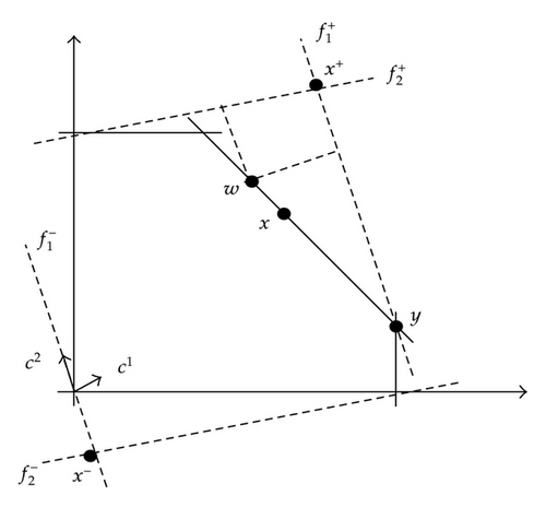
Example 3.1 (Graphical Example). Consider Figure 1 in which x+ is the inverse image of f+ and x− is the inverse image of f−.
Also, consider that w and y are the optimal solutions of models (3.12) and (3.15), respectively.
w is a solution whose criterion vector is closest to f+ and y is a solution whose criterion vector is furthest to f−.
Point x which is obtained by model (3.18) is a solution whose criterion vector is closest to f+ and furthest to f− and therefore is a compromise solution.
Step 6 (decision phase). The compromise solution x(h) is presented to the decision maker, who compares objective vector f(x(h)) with the positive ideal criterion vector f+ and negative ideal criterion vector f−. This decision phase has the following steps.
Substep 6.1. If all components of f(x(h)) are satisfactory, stop with (x(h), f(x(h))) as the final solution and x(h) is the best compromise solution. Otherwise go to Substep 6.2.
Substep 6.2. If all components of f(x(h)) are not satisfactory, then terminate the interactive process and use other methods to search for the best compromise solutions. Otherwise go to Substep 6.3.
Substep 6.3. If some components of f(x(h)) are satisfactory and others are not, the DM must relax an objective fj(x) to allow an improvement of the unsatisfactory objectives in the next iteration. If the decision maker cannot find an objective to sacrifice, then the interactive process will be terminated and other methods have to be used for identifying the best compromise solution, otherwise, the DM gives Δfj as the amount of acceptable relaxation. Δfj is the maximum amount of fj(x) we are willing to sacrifice. Now go to Substep 6.4.
Substep 6.4. Define a new reduced feasible region as follows:
4. Numerical Example
In this section we investigate the capability of the proposed method.
4.1. The Problem Description
4.2. Solve with the Proposed Method
In order to find a satisfactory solution, we carry out the following steps.
Iteration Number 1
Step 1 (first pay-off table). The first pay-off table of the problem is as shown in Table 3.
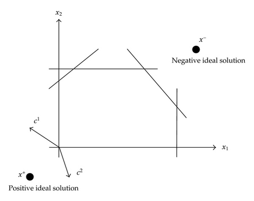
Table 3 is constructed using formula (3.1). Figure 2 shows the feasible region and objectives. Also in Figure 2 we can see the negative ideal solution and positive ideal solution.
Step 2 (second pay-off table). The second pay-off table of the problem is as shown in Table 4.
Step 3 (obtain the first group of weights). Since and m1 = −30 and c11 = −5, c12 = 2, then from formula (3.5) we have
Step 4 (obtain the second group of weights). Since and n1 = 3 and c11 = −5, c12 = 2, then from formula (3.8) we have
Step 5 (calculation phase). Now we can start the iteration process. Therefore we have the following steps.
Substep 5.6 (find the closest criterion vector to positive ideal). We can obtain a criterion vector which is closest to the positive ideal one by solving model (3.12) as follows:
Substep 5.7 (find the furthest criterion vector to negative ideal). We can obtain a criterion vector which is furthest to the negative ideal one by solving model (3.15) as follows:
Substep 5.8 (obtain a compromise solution). We can obtain a criterion vector which is closest to positive ideal and furthest to negative ideal by solving model (3.18) as follows:
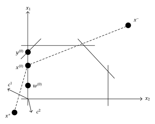
Step 6 (decision phase). The results x(0) = (0,2.013) and f(x(0)) = {4.026, −8.052} are shown to the decision maker. Suppose the solution is not satisfied as f2(x(0)) = −8.052 is too small. Suppose f1(x) can be sacrificed by 2 units, or Δf1 = 2. Then the new search space is given by
In Figure 3 we can see the obtained solutions from iteration 1. Specially we can see the compromise solution obtained from iteration 1 that is denoted by x(0).
| f1 | f2 | Solution | Vector | |
|---|---|---|---|---|
| f1 | f12 = −12 | |||
| f2 | f21 = −30 |
| f1 | f2 | Solution | Vector | |
|---|---|---|---|---|
| f1 | z12 = 6 | |||
| f2 | z21 = 3 |
Iteration Number 2 It is obvious that , and we go to Step 5. It is done in three steps.
Substep 6.6 (find the closest criterion vector to positive ideal). In this step we solve model (3.7) as follows:
Substep 6.7 (find the furthest criterion vector to negative ideal). Solve model (3.7) as follows:
Substep 6.8 (obtain a compromise solution). In order to obtain a criterion vector which is closest to the positive ideal and furthest to the negative ideal, we solve model (3.7) as follows:
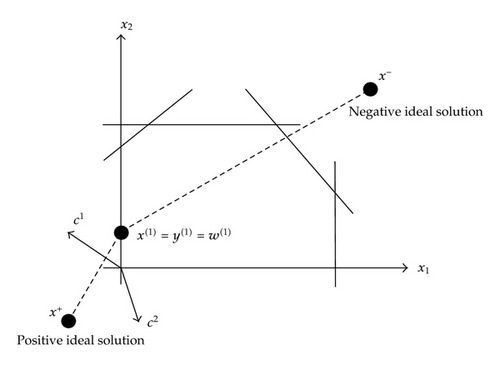
Note that x(1) is the point in feasible region whose criterion vector is closet to criterion vector w(1) and y(1) and therefore whose criterion vector has minimum distance to positive ideal and has maximum distance to negative ideal one.
In Figure 4 we can see the obtained solutions from iteration 2. Specially we can see the compromise solution and other solutions obtained from iteration 1 coincide. The compromise solution that is denoted by x(1) is also the preferred solution.
According to the behavioral assumptions of the STEM method (discussed in decision phase), the decision maker should be satisfied with the solution x(1); otherwise, there would be no best compromise solution.
For this two-objective problem, this conclusion may be acceptable as f1(x) can be sacrificed by as much as 2 units from f1(x(0)), and his sacrifice has been fully used to benefit the objective f2(x). In general, such conclusion may not be rational for problems having more than two objectives. In such circumstances, whether the decision maker is satisfied with a solution depends on the range of solutions he has investigated. Also, the sacrifices of multiple objectives should also be investigated in addition to the sacrifice of a single objective at each iteration.
4.3. Solving with the Classic STEM Method
Suppose we want to solve the above problem with the classic STEM method. Therefore the iterations of solving this problem are as shown in Table 5.
| Iteration (h) | x(h) | f(x(h)) |
|---|---|---|
| 1 | (0.000,0.452) | (0.904, −1.808) |
| 2 | (0.000,0.952) | (1.904, −3.808) |
In iteration 2, we set Δf1 = 2. By comparing with the results of proposed method, we can see that the optimal objective is further to the negative ideal objective.
5. Conclusion
The suggested method in this paper improves the STEM method by finding a point in reduced feasible region whose criterion vector is closest to the positive ideal criterion vector and furthest to the negative ideal criterion vector. Therefore the presented method increases the rate of satisfactoriness of the obtained solution.
Acknowledgment
The author is grateful to the helpful comments and suggestions made by anonymous referees.


