

Efficient Boundary Extraction from Orthogonal Pseudo-Polytopes: An Approach Based on the nD-EVM
Abstract
This work is devoted to contribute with two algorithms for performing, in an efficient way, connected components labeling and boundary extraction from orthogonal pseudo-polytopes. The proposals are specified in terms of the extreme vertices model in the n-dimensional space (nD-EVM). An overview of the model is presented, considering aspects such as its fundamentals and basic algorithms. The temporal efficiency of the two proposed algorithms is sustained in empirical way and by taking into account both lower dimensional cases (2D and 3D) and higher-dimensional cases (4D and 5D).
1. Introduction
The extreme vertices model in the n-dimensional space (nD-EVM) is a representation scheme whose dominion is given by the n-dimensional orthogonal pseudo-polytopes, that is, polytopes that can be seen as a finite union of iso-oriented nD hyperboxes (e.g., hypercubes). The fundamental notions of the model, for representing 2D and 3D-OPPs, were originally established by Aguilera and Ayala in [1, 2]. Then, in [3], it was formally proved the model is capable of representing and manipulating nD-OPPs. The nD-EVM has a well-documented repertory of algorithms (see [1, 3–7]) for performing tasks such as Regularized Boolean operations, set membership classification, measure interrogations (content and boundary content), morphological operations (e.g., erosion and dilation), geometrical and topological interrogations (e.g., discrete compactness), among other algorithms currently being in development. Furthermore, conciseness, in terms of spatial complexity, is one the nD-EVM’s main properties, because the model only requires storing a subset of a polytope’s vertices, the extreme vertices, which finally provides efficient temporal complexity of our algorithms. Sections 2 and 3 are summaries of results originally presented in [1, 3]. For the sake of brevity, and because we aim for a self-contained paper, some propositions are only enunciated. Their corresponding proofs and more specific details can be found in [1, 3]. In Section 2, the main concepts and basic algorithms behind the nD-EVM are described, while Section 3 presents an algorithm for extracting forward and backward differences of an nD-OPP.
- (i)
Methods that require multiple passes over the data: the scanning step is repeated successively until each pixel has a definitive label.
- (ii)
Two-pass methods: they scan the image once to assign temporal labels. A second pass has the objective of assigning the final labels. They make use of lookup lists or tables in order to model relationships between temporal and/or equivalent labels [9].
- (iii)
Methods that use equivalent representations of the data: their strategy is based on using a more suitable representation based on hierarchical tree structures (quadtrees, octrees, etc.) instead of the image’s raw data in order to speed up the labeling [10, 14].
- (iv)
Parallel algorithms.
In [7], Rodríguez and Ayala describe an EVM-based algorithm for connected components labeling. It works specifically for 2D and 3D-OPPs. First, they obtain a particular partitioning from the 3D-EVM known as ordered union of disjoint boxes (OUODB), which is, in fact, a special kind of cell decomposition [7]. Then, once the OUODB partition has been achieved, it follows a process which is based in the two-pass approach. We take into account some ideas presented by Rodríguez and Ayala, but our proposal deals with a higher-dimensional context, that is, with nD-OPPs, and it works directly with their corresponding nD-EVM representations.
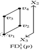
Section 5 describes the second contribution of this work: a methodology for extracting kD boundary elements from an nD-OPP represented through the nD-EVM. It is well known that a boundary model for a 3D solid object is a description of the faces, edges, and vertices that compose its boundary together with the information about the connectivity between those elements [15]. However, the boundary representations can be recursively applied not only to solids, surfaces, or segments but to n-dimensional polytopes [16]. For Putnam and Subrahmanyan, a polytope’s boundary representation can be seen as a boundary tree [17]. In the tree, each node is split into a component for each element that it bounds. An element (vertex, edge, etc.) will be represented several times inside the tree, one for each boundary that it belongs to. See Figure 1 for a cube’s boundary tree.

The way we extract kD boundary elements from an nD-OPP represented through the nD-EVM will be reminiscent to the reconstruction of the boundary tree associated with such nD-OPP. Moreover, our methodology is strongly sustained in the use of our proposed connected components labeling algorithm (Section 4) and the procedures described in Sections 2 and 3. Some study cases will be presented in order to appreciate the information our proposed procedure can share. Finally, in Section 6, we determine, in empirical way, the time complexity of the algorithm presented in Section 5 in order to provide evidence of its efficiency specifically when higher-dimensional nD-OPPs are considered.
2. The Extreme Vertices Model in the n-Dimensional Space (nD-EVM)
In Section 2.1, some conventions and preliminary background related directly with orthogonal polytopes will be introduced. In Section 2.2, the foundations of the nD-EVM will be established. Section 2.3 presents some basic algorithms under the EVM.
2.1. The n-Dimensional Orthogonal Pseudo-Polytopes (nD-OPPs)
- (a)
A singular n-dimensional hyperbox in ℝn is given by the continuous function In : [0,1] n → [0,1] n such that In(x) = x.
- (b)
For all i, 1 ≤ i ≤ n, if x ∈ [0,1] n−1, then the two singular (n − 1)D hyperboxes and are given by
- (c)
A general singular k-dimensional hyperbox in the closed set A ⊂ ℝn is defined as the continuous function c : [0,1] k → A.
- (d)
Given a general singular nD hyperbox c the composition defines an (i, α)-cell.
- (e)
The orientation of an (n − 1)D cell is given by (−1) α+i, while an (n − 1)D oriented cell is given by the scalar-function product .
- (f)
A formal linear combination of singular general kD hyperboxes, 1 ≤ k ≤ n, for a closed set A is called a k-chain.
- (g)
Given a singular nD hyperbox In, the (n − 1)-chain, called the boundary of In, is defined as
- (h)
For a singular general nD hyperbox c, we define the (n − 1)-chain, called the boundary of c, by
- (i)
The boundary of an n-chain ∑ci, where each ci is a singular general nD hyperbox, is given by
The first part of the conjunction establishes that the intersection between all the nD general singular hyperboxes is the origin, while the second part establishes that there are not overlapping nD hyperboxes. Finally, we will say an n-dimensional orthogonal pseudopolytope p, or just an nD-OPP p, is an n-chain composed by nD hyperboxes arranged in such way that by selecting a vertex, in any of these hyperboxes, it describes a combination of nD hyperboxes composed up to 2n hyperboxes.
2.2. nD-EVM’s Fundamentals
Let c be a combination of hyperboxes in the n-dimensional space. An odd adjacency edge of c, or just an odd edge, will be an edge with an odd number of incident hyperboxes of c. Conversely, if an edge has an even number of incident hyperboxes of c, it will be called even adjacency edge or just an even edge. A brink or extended edge is the maximal uninterrupted segment, built out of a sequence of collinear and contiguous odd edges of an nD-OPP. By definition, every odd edge belongs to brinks, whereas every brink consists of m edges, m ≥ 1, and contains m + 1 vertices. Two of these vertices are at either extreme of the brink and the remaining m − 1 are interior vertices. The ending vertices of all the brinks in p will be called extreme vertices of an nD-OPP p and they are denoted as EV(p). Finally, we have that any extreme vertex of an nD-OPP, n ≥ 1, when is locally described by a set of surrounding nD hyperboxes, has exactly n incident linearly independent odd edges.
Given an nD-OPP, we say the extreme vertices model of p, denoted by EVMn(p), is defined as the model as only stores to all the extreme vertices of p. We have that EVMn(p) = EV(p) except by the fact that coordinates of points in EV(p) are not necessarily sorted. In general, it is always assumed that coordinates of extreme vertices in the extreme vertices model of an nD-OPP p, EVMn(p), have a fixed coordinates ordering. Moreover, when an operation requires manipulating two EVMs, it is assumed both sets have the same coordinates ordering.
- (i)
Let be an (n − 1)D cell embedded in the nD space. will denote the projection of the cell onto an (n − 1)D space embedded in nD space whose supporting hyperplane is perpendicular to Xj-axis; that is, .
- (ii)
Let v = (x1, …, xn) a point in ℝn. The projection of that point in the (n − 1)D space, denoted by πj(v), is given by .
- (iii)
Let Q be a set of points in ℝn. The projection of the points in Q, denoted by πj(Q), is defined as the set of points in ℝn−1 such that πj(Q) = {p ∈ ℝn−1 : p = πj(x), x ∈ Q ⊂ ℝn}.
In all the three above cases, is the coordinate corresponding to Xj-axis to be suppressed.
For an nD-OPP p, we will say that npi denotes the number of distinct coordinates present in the vertices of p along Xi-axis, 1 ≤ i ≤ n. Let be the kth (n − 1)D extended hypervolume, or just a (n − 1)D Couplet, of p which is perpendicular to Xi-axis, 1 ≤ k ≤ npi.
A slice is the region contained in an nD-OPP p between two consecutive couplets of p. will denote to the kth slice of p, which is bounded by and , 1 ≤ k < npi. A section is the (n − 1)D-OPP, n > 1, resulting from the intersection between an nD-OPP p and a (n − 1)D hyperplane perpendicular to the coordinate axis Xi, n ≥ i ≥ 1, which dose not coincide with any (n − 1)D-couplet of p. A section will be called external or internal section of p if it is empty or not, respectively. will refer to the kth section of p between and , 1 ≤ k < npi. Moreover, and will refer to the empty sections of p before and after , respectively.
The projection of the set of (n − 1)D couplets, , 1 ≤ i ≤ n, of an nD-OPP p can be obtained by computing the regularized XOR (⊗*) between the projections of its previous and next sections; that is, . On the other hand, the projection of any section, , of an nD-OPP p can be obtained by computing the regularized XOR between the projection of its previous section, , and the projection of its previous couplet . Or, equivalently, by computing the regularized XOR of the projections of all the previous couplets; that is, .
2.2.1. The Regularized XOR Operation on the nD-EVM
- (i)
,
- (ii)
.
2.2.2. The Regularized Boolean Operations on the nD-EVM
Let p and q be two nD-OPPs and r = p op*q, where op* is in {∪*, ∩*, −*, ⊗*}. Then, . This implies a regularized Boolean operation, op*, where op* ∈ {∪*, ∩*, −*, ⊗*}, over two nD-OPPs p and q, both expressed in the nD-EVM, can be carried out by means of the same op* applied over their own sections, expressed through their extreme vertices models, which are (n − 1)D-OPPs. This last property leads to a recursive process, for computing the regularized Boolean operations using the nD-EVM, which descends on the number of dimensions. The base or trivial case of the recursion is given by the 1D-Boolean operations which can be achieved using direct methods. The XOR operation can also be performed according to the result described in the above subsection.
2.3. Basic Algorithms for the nD-EVM
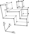
Before going any further, we say XA-axis is the nD space’s coordinate axis associated to the first coordinate present in the vertices of EVMn(p). For example, given coordinates ordering X1X2X3, for a 3D-OPP, then XA = X1.
The following primitive operations are, in fact, based in those originally presented in [1] see Algorithm 1.
-
Algorithm 1: Basic procedures under the EVM.
-
Output: An empty nD-EVM.
-
Procedure InitEVM( )
-
{ Returns the empty set. }
-
Input: An (n − 1)D-EVM hvl embedded in nD space.
-
Input/Output: An nD-EVM p
-
Procedure PutHvl(EVM hvl, EVM p)
-
{ Appends an (n − 1)D couplet hvl, perpendicular to XA-axis, to p. }
-
Input: An nD-EVM p
-
Output: An (n − 1)D-EVM embedded in (n − 1)D space.
-
Procedure ReadHvl(EVM p)
-
{ Extracts next (n − 1)D couplet perpendicular to XA-axis from p. }
-
Input: An nD-EVM p
-
Output: A Boolean.
-
Procedure EndEVM(EVM p)
-
{ Returns true if the end of p along XA-axis has been reached. }
-
Input/Output: An (n − 1)D-EVM p embedded in (n − 1)D space.
-
Input: A coordinate coord of type CoordType
-
(CoordType is the chosen type for the vertex coordinates)
-
Procedure SetCoord(EVM p, CoordType coord)
-
{ Sets the XA-coordinate to coord on every vertex of the (n − 1)D
-
couplet p. For coord = 0, it performs the projection πA(p). }
-
Input: An (n − 1)D-EVM p embedded in nD space.
-
Output: A CoordType
-
Procedure GetCoord(EVM p)
-
{ Gets the common XA coordinate of the (n − 1)D couplet p. }
-
Input: An nD-EVM p.
-
Output: A CoordType
-
Procedure GetCoordNextHvl(EVM p)
-
{ Gets the common XA coordinate of the next available (n − 1)D couplet of p. }
-
Input: Two nD-EVMs p and q.
-
Output: An nD-EVM
-
Procedure MergeXor(EVM p, EVM q)
-
{ Applies the ordinary Exclusive OR operation to the vertices of
-
p and q and returns the resulting set. }
-
Input: An (n − 1)D-EVM corresponding to section S.
-
An (n − 1)D-EVM corresponding to couplet hvl.
-
Output: An (n − 1)D-EVM.
-
Procedure GetSection(EVM S, EVM hvl)
-
{ return MergeXor(S, hlv) }
-
Input: An (n − 1)D-EVM corresponding to section Si.
-
An (n − 1)D-EVM corresponding to section Sj.
-
Output: An (n − 1)D-EVM.
-
Procedure GetHvl(EVM Si, EVM Sj)
-
{ return MergeXor (Si, Sj) }
-
Input: Two nD-EVMs p and q.
-
The Boolean Operation op to apply over p and q.
-
The number n of dimensions.
-
Output: An nD-EVM.
-
Procedure BooleanOperation(EVM p, EVM q, BooleanOperator op, int n)
-
{ Returns as output an nD-OPP r, codified as an nD-EVM, such that
-
r = p op*q. }
As can be observed, algorithms MergeXor, GetSection, and GetHvl are clearly sustained in the results presented in Section 2.2. The algorithm GetSection, via MergeXor algorithm, returns the projection of the next section of an nD-OPP between its previous section and couplet [1, 3]. On the other hand, the algorithm GetHvl returns the projection of the couplet between consecutive input sections Si and Sj [1, 3].
- (i)
The sequence of sections from p and q, perpendicular to XA-axis, are obtained first.
- (ii)
Then, every section of r can recursively be computed as
- (iii)
Finally, r’s couplets can be obtained from its sequence of sections, perpendicular to XA-axis.
In fact, BooleanOperation can be implemented in a wholly merged form in which it only needs to store one section for each of the operands p and q (sP and sQ, resp.), and two consecutive sections for the result r (sRprev and sRcurr) [1]. The idea is to consider a main loop that gets sections from p and/or q, using function GetSection. These sections, sP and sQ, are recursively processed to compute the corresponding section of r, sRcurr. Since r’s two consecutive sections, sRprev and sRcurr, are kept, then the projection of the resulting couplet, is obtained by means of function GetHvl, and then, it is correctly positioned in r’s EVM by procedure SetCoord [1]. When the end of one of the polytopes p or q is reached, then the main loop finishes, and the remaining couplets of the other polytope are either appended or not to the resulting polytope r depending on the Boolean operation considered. More specific details about this implementation of BooleanOperation algorithm can be found in [1] or [3].
3. Forward and Backward Differences of an nD-OPP
One interesting characteristic, described in [1], of forward and backward differences of a 3D-OPP, is that forward differences are the sets of faces, on a couplet, whose normal vectors point to the positive side of the coordinate axis perpendicular to such couplet. Similarly, backward differences are the sets of faces, on a couplet, whose normal vectors point to the negative side of the coordinate axis perpendicular to such couplet. By this way, it is provided a procedure for obtaining the correct orientation of faces in a 3D-OPP when it is converted from 3D-EVM to a boundary representation.
In the context of an nD-OPP p, there are methods to identify normal vectors in the (n − 1)D cells included in p’s boundary. For example, simplicial combinatorial topology provides methodologies assuming a polytope is represented under a simplexation. Such methods operate under the fact the n + 1 vertices of an nD simplex are labeled and sorted. Such sorting corresponds to an odd or an even permutation. By taking n vertices from the n + 1 vertices of the nD simplex, we get the vertices corresponding to one of its (n − 1)D-cells. In this point, usually, a set of entirely arbitrary rules are given to determine the normal vector to such (n − 1)D cells; see for example, [19, 20]. Such rules establish, according to the parity of the permutation, if the assigned normal vector points towards the interior of the polytope or outside of it.
On the other hand, there are works that consider the determination of normal vectors by taking into account properties of the cross product and the vectors that compose the basis of nD space. For example, Kolcun [21] provides one of such methodologies; however, it is also dependent of polytopes are represented through a simplexation. In this last sense, forward and backward differences will provide us a powerful tool, because, in fact, given an nD-OPP p, forward differences are the sets of (n − 1)D cells lying on , whose normal vectors point to the positive side of the coordinate axis Xi, while backward differences are the sets of (n − 1)D cells also lying on but whose normal vectors point to the negative side of the coordinate Xi-axis.
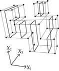
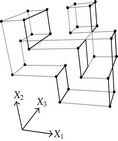
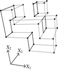
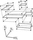
Figure 2 shows a 3D-OPP and its corresponding sets of 2D-couplets perpendicular to X1, X2, and X3-axes (Figures 2(b), 2(c), 2(d)). According to Figure 2(a), the OPP has 5 non-extreme vertices which are marked in white. Three of them have four coplanar incident odd edges; another one has six incident odd edges, and the last one has exactly two incident collinear odd edges. The remaining vertices, actually the extreme vertices, have exactly three linearly independent odd edges. Table 1 shows the extraction, for the 3D-OPP shown in Figure 2(a), of its faces and their correct orientation through forward and backward differences. The first row shows sections perpendicular to X1-axis. Through them, we compute forward differences to in order to obtain the faces whose normal vector points towards the positive side of X1-axis. On the other hand, these same sections share us to compute backward differences to , which are composed by the set of faces whose normal vector points towards the negative side of X1-axis. In a similar way, the remaining two rows of Table 1 show sections perpendicular to X2 and X3-axes and their respective forward and backward differences.
| Sections | Forward differences | Backward differences |
|---|---|---|
 |
 |
 |
 |
 |
 |
 |
 |
 |


An algorithm for computing forward and backward differences consists of obtaining projections of sections of the input polytope and processing them through BooleanOperation algorithm by computing regularized difference between two consecutive sections. Algorithm 2 implements these simple ideas in order to compute the forward and backward differences in an nD-OPP p represented through the nD-EVM. Its output will consist of two sets: the first set FD contains the (n − 1)D-EVMs corresponding to forward differences in p, while the second set BD contains the (n − 1)D-EVMs corresponding to backward differences in p. Algorithm 2 will be useful when we describe our procedure for extracting kD boundary elements of an nD-OPP which is represented through the nD-EVM. Such procedure will be described in Section 5.
-
Algorithm 2: Computing forward and backward differences in a polytope p represented through an nD-EVM.
-
Input: An nD-EVM p.
-
The number n of dimensions.
-
Output: A set FD containing the (n − 1)D-EVMs of Forward Differences in p.
-
A set BD containing the (n − 1)D-EVMs of Backward Differences in p.
-
Procedure GetForwardBackwardDifferences(EVM p, int n)
-
FD = ∅ // FD will store (n − 1)D-EVMs corresponding to Forward Differences.
-
BD = ∅ // BD will store (n − 1)D-EVMs corresponding to Backward Differences.
-
EVM hvl // Current couplet.
-
EVM Si, Sj // Previous and next sections about hvl.
-
EVM FDcurr // Current Forward Difference.
-
EVM BDcurr // Current Backward Difference.
-
hvl = InitEVM( )
-
Si = InitEVM( )
-
Sj = InitEVM( )
-
while(Not(EndEVM(p)))
-
hvl = ReadHvl(p)// Read next couplet.
-
Sj = GetSection(Si, hvl)
-
FDcurr = BooleanOperation(Si, Sj, Difference, n − 1)
-
BDcurr = BooleanOperation(Sj, Si, Difference, n − 1)
-
FD = FD ∪ {FDcurr}// The new computed Forward Difference is added to FD.
-
BD = BD ∪ {BDcurr}// The new computed Backward Difference is added to BD.
-
Si = Sj
-
end-of-while
-
return {FD, BD}
-
end-of-procedure
4. A Connected Components Labeling Algorithm under the nD-EVM
- (i)
It processes only two consecutive slices of p at a time. In fact, such slices are not explicitly manipulated but their corresponding representative (n − 1)D sections.
- (ii)
The algorithm descends recursively over the number of dimensions in such way that it is determined for each (n − 1)D section of p its corresponding (n − 2)D components. By this way, the (n − 2)D components of two consecutive (n − 1)D sections are manipulated and used for determining the labels to assign.
The idea behind the proposed methodology considers to process sequentially each (n − 1)D section of p. Let Sj be the current processed section of p. We obtain, via a recursive call, its (n − 1)D components. Let Si be the section before Sj. For each (n − 1)D component cSj in Sj and for each (n − 1)D component cSi in Si, it is performed their regularized intersection cSj∩*cSi. According to the result, one of three cases can arise.
Case 1. (i) If the intersection is not empty and cSj does not belong to any component of p, then cSj is added to the component of p, where the current component of Si, cSi, belongs.
Case 2. (i) If the intersection is not empty but cSj is already associated to a component of p, then such component and the component where cSi is contained are united to form only one new component for p. It could be the case that both components to unite are, in fact, the same. In this situation, no action is performed. On the other hand, if the union is achieved, then all the references pointing to the original nD components where cSi and cSj belonged must be updated in order to point to the new component.
Case 3. (i) If the intersection with all components of Si is empty, then cSj does not belong to any of the currently identified components of p. Therefore, cSj belongs to, and starts, a new nD component.
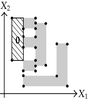
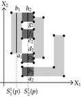
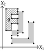
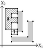
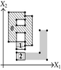
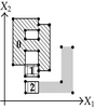
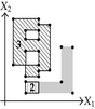
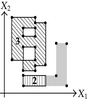
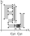
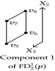
Tables 2 and 3 show an example where the above ideas are applied on a 2D-OPP. Such OPP is composed of 22 extreme vertices and has five internal sections which are perpendicular to X1-axis. Once all sections are processed, it is determined the existence of two components.
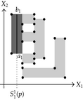 |
The projection of section has the 1D component . Because is an empty section. Then, Case 3: belongs to the new component 0. |
 |
|---|---|---|
 |
The projection of section has four 1D components: , , , and . | |
|
 |
|
|
 |
|
|
 |
|
|
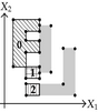 |
| Projection of section has two 1D components: and . | ||
|---|---|---|
 |
|
 |
|
 |
|
|
 |
|
|
 |
|
| The projection of section is composed by segment . | ||
 |
|
 |
| The projection of section is composed by segment . | ||
 |
|
 |
A more specific implementation of our procedure is given in Algorithm 3. In order to distinguish between Cases 1 and 2, the algorithm uses a Boolean flag (withoutComponent). When Case 1 is achieved, then cSj, the current component of section Sj, is already associated to a component of p. Therefore, the flag’s value is inverted for indicating this last property and, for instance, sharing that only Case 2 could be reached in the subsequent iterations. If for all components of Si, the section before Sj, the intersection with cSj was empty, then the flag never changed its original value. In this way, Case 3 can be identified.
-
Algorithm 3: Connected component labeling over an nD-OPP expressed in the nD-EVM.
-
Input: An nD-OPP p.
-
The number n of dimensions.
-
Output: A list containing the EVMs which describe the nD components of p.
-
Procedure ConnectedComponentsLabeling(EVM p, int n)
-
if(n = 1) then
-
return ConnectedComponentsLabeling1D(p) // Base case.
-
else
-
EVM hvl // Current (n − 1)D couplet of p.
-
EVM Si, Sj // Previous and next (n − 1)D sections about hvl.
-
Si = InitEVM( )
-
List components Si // The (n − 1)D components of section Si.
-
List indexes Si // A list of indexes.
-
List components Sj // The (n − 1)D components of section Sj.
-
List indexes Sj // A list of indexes.
-
List componentsP // The nD components of input polytope p.
-
CoordType currCoord = getCoordNextHvl(p)
-
hvl = ReadHvl(p)
-
CoordType nextCoord = getCoordNextHvl(p)
-
while(Not(EndEVM(p)))
-
Sj = GetSection(Si, hvl)
-
components Sj = ConnectedComponentsLabeling (Sj, n − 1) // Recursive call.
-
for(int j = 0, j < Size(components Sj), j = j + 1)
-
EVM cSj = components Sj(j)
-
boolean withoutComponent = true
-
for(int i = 0, i < Size(components Si), i = i + 1)
-
EVM cSi = components Si(i)
-
EVM c = BooleanOperation(cSj,cSi, Intersection, n − 1)
-
if(Not(IsEmpty(c)) and (withoutComponent = true)) then
-
// CASE 1
-
withoutComponent = false
-
List componentToUpdate = componentsP(indexes Si(i))
-
Append(componentToUpdate, {cSj, currCood, nextCoord})
-
Append(indexes Sj, indexes Si(i))
-
else if(Not(IsEmpty(c)) and (withoutComponent = false)) then
-
// CASE 2
-
if(indexes Si(i)≠ indexes Sj(j)) then
-
List component1 = componentsP(indexes Si(i))
-
List component2 = componentsP(indexes Sj(j))
-
for(int k = 0, k < Size(component1), k = k + 1)
-
Append(component2, component1(k))
-
end-of-for
-
Update(componentsP, indexes Si(i), NULL)
-
for(int k = 0, k < Size(indexes Si), k = k + 1)
-
if(indexes Si(k) = indexes Si(i)) then
-
Update(indexes Si, k, indexes Sj(j))
-
end-of-if
-
end-of-for
-
for(int k = 0, k < Size(indexes Sj), k = k + 1)
-
if(indexes Sj(k) = indexes Si(i)) then
-
Update(indexes Sj, k, indexes Sj(j))
-
end-of-if
-
end-of-for
-
Update(indexes Si, i, indexes Sj(j))
-
end-of-if
-
end-of-if
-
end-of-for
-
if(withoutComponent = true) then
-
// CASE 3
-
List newComponent
-
Append(newComponent, {cSj, currCoord, nextCoord})
-
Append(componentsP, newComponent)
-
Append(indexes Sj, Size(componentsP) - 1)
-
end-of-if
-
end-of-for
-
Si = Sj
-
components Si = components Sj
-
indexes Si = indexes Sj
-
currCoord = GetCoordNextHvl(p)
-
hvl = ReadHvl(p) // Read next couplet.
-
nextCoord = GetCoordNextHvl(p)
-
end-of-while
-
// End of sections’ processing.
-
int i = 0
-
while(i < Size(componentsP))
-
if(componentsP(i) = NULL) then
-
Remove(componentsP, i)
-
i = i − 1
-
else
-
List currentListOfSections = componentsP(i)
-
EVM evmComponent = getEVMforListOfSections(currentListOfSections, n)
-
Update(componentsP, i, evmComponent)
-
end-of-if
-
i = i + 1
-
end-of-while
-
return componentsP
-
end-of-if
-
end-of-procedure
- (i)
Size (list): returns the number of elements in the list.
- (ii)
List (i): returns the element at position i of the list, 0 ≤ i < Size(list).
- (iii)
Update (list, i, nV): the list is updated by substituting element in position i with the new element nV.
- (iv)
Append (list, v): an element v is appended at the end of the list.
- (v)
Insert (list, i, v): an element v is inserted at position i of the list.
- (vi)
Remove (list, i): it is removed from the list the element at position i.
- (vii)
IndexOf (list, v): returns a negative integer if v is not present in the list. Otherwise, an index between 0 and Size (list)-1 is returned indicating the first occurrence of v.
- (viii)
DeleteAll (list): deletes all the elements contained in the list.
- (i)
componentsSj (componentsSi): the (n − 1)D components of section Sj(Si). The (n − 1)D-EVM associated to the jth (ith) component of section Sj(Si) is obtained via componentsSj( j) (componentsSi( i)).
- (ii)
indexesSj (indexesSi): a list of indexes. k1 = indexesSj(j) (k2 = indexesSi(i)) denotes the jth (ith) component of section Sj(Si) belongs to the k1th (k2th) component of nD-OPP p.
- (iii)
componentsP: the components of input nD-OPP p. components( k) returns a list of (n − 1)D sections which describe the kth nD component of p.
- (i)
In Case 1, componentsP(indexesSi( i)) returns the component of p, where cSi belongs. cSj is incorporated to such component by appending it in such list. Finally, via Append(indexesSj, indexesSi( i)), it is now established that cSj belongs to the same component than cSi, because they have the same component’s index.
- (ii)
In Case 2, we obtain the components, where cSi and cSj belong through componentsP(indexesSi(i)) and componentsP(indexesSj(j)) (if indexesSi(i) and indexesSj(j) are equal, then, as commented previously, no action is performed). All the elements in the first component are transferred to the second component. The position where the first component resided in the list componentsP is now updated to NULL. Via, Update(indexesSi, i, indexesSj(j)), it is established that cSi belongs to the same component like cSj. Finally, it must be verified if there are (n − 1)D components of Si and Sj whose value in indexesSi and indexesSj refers to the now nullified position in componentsP. If it is the situation, then their indexes must be updated with the value in indexesSj(j).
- (iii)
In Case 3, a new component for nD-OPP p is created. The new list, containing only to cSj, is appended in list componentsP. The value given by the size of list componentsP minus one is appended in list indexesSj. Such value corresponds to the component’s index for cSj.
When the algorithm finishes the processing of sections, each list in componentsP is a list of (n − 1)D sections or a NULL element. If a NULL element is found, then it must be removed. Otherwise, we obtain the corresponding nD-EVM, which at its time corresponds to a component of the input nD-OPP p. It is possible the (n − 1)D sections contained in a given list are not correctly ordered. With the purpose of determining the correct sequence, in Algorithm 3, when a (n − 1)D-OPP is appended, the common XA coordinates of the previous and next couplets are also introduced with it.
- (i)
C1 = [0,1] × [0,1] × [0,1] × [0,1] × [0,1],
- (ii)
C2 = [0,1] × [1,2] × [0,1] × [0,1] × [0,1],
- (iii)
C3 = [0,1] × [2,3] × [0,1] × [0,1] × [0,1],
- (iv)
C4 = [1,2] × [2,3] × [0,1] × [0,1] × [0,1],
- (v)
C5 = [2,3] × [2,3] × [1,2] × [1,2] × [1,2],
- (vi)
C6 = [3,4] × [2,3] × [0,1] × [1,2] × [1,2].


Previously, we mentioned hypercubes C5 and C6 shared a 3D volume. When computing regularized intersection between and (their corresponding sections in q) the result was the empty set. This is due to the use of regularized boolean operations: operations between nD polytopes must be dimensionally homogeneous; that is, they must produce as result another nD polytope or the null object [22]. Hypercubes C5 and C4 shared a (1D) edge, but the regularized intersection between their corresponding sections, in q, and , also produced a null object. A distinct situation arises when the regularized intersection between and is analyzed: Algorithm 3 determined that they are associated with the same component.
The above example has illustrated a property of Algorithm 3. When the foundations behind our method were established, it was commented the algorithm process, not in an explicit way, consecutive slices of the input polytope p. Each nD slice of p has its corresponding representative (n − 1)D section for which Algorithm 3 determines its corresponding (n − 1)D components. Let c1 and c2 be nonempty (n − 1)D components such that c1 is associated to (n − 1)D section , while c2 is associated to (n − 1)D section . The fact that c1 and c2 have empty regularized intersection implies (1) that their corresponding nD regions are disjoint and, therefore, they have null adjacencies, or (2) that some parts of its corresponding slices have a kD adjacency; that is, some kD elements, k = 0,1, 2, …, n − 2, are, completely or partially, shared. In both cases, Algorithm 3 uses this kind of adjacencies, via the result of regularized intersection between c1 and c2, for determining that the corresponding nD regions are disjoint and, for instance, associate them with different components. Hence, a nD component shared by Algorithm 3 corresponds to those parts of the input nD-OPP that are united via (n − 1)D adjacencies. The way Algorithm 3 breaks a polytope will be very useful in the following sections, specifically when we present our methodology for identifying kD boundary elements.
5. Extracting kD Boundary Elements from an nD-OPP
This section presents the second main contribution of this work. As commented in Section 1, the way we extract kD boundary elements from an nD-OPP represented through the nD-EVM will be reminiscent to the reconstruction of the boundary tree associated to such nD-OPP. According to Section 3, forward and backward differences can be computed through Algorithm 2. In fact, all and from an nD-OPP are (n − 1)D-OPPs embedded in (n − 1)D space, because the projection operator is used in their corresponding definitions: and . If such forward and backward differences were computed through our proposed algorithm, then they are expressed as and . If we apply again Algorithm 2 to such (n − 1)D-OPPs, we will get new forward and backward differences that correspond to the (n − 2)D oriented cells on the boundary of such (n − 1)D-OPPs. These new forward and backward differences are themselves (n − 2)D-OPPs represented through the EVM. Hence, by applying again Algorithm 2 to them, we obtain their associated (n − 3)D oriented cells grouped as forward and backward differences. This procedure generates a recursive process which descends in the number of dimensions. In each recursivity level, we obtain forward and backward differences associated to the input kD-OPPs, 1 ≤ k ≤ n. The base case is reached when n = 1. In this situation, the boundary of a 1D-OPP is described by the beginning and ending extreme vertices of each one of its composing segments.
Algorithm 4 implements the above-proposed ideas in order to identify and to extract kD boundary elements from a nD-OPP. Input parameters for our algorithm require the EVM associated with the input nD-OPP p, the number k of dimensions, and a list, where the boundary elements of p are going to be stored. Such a list, called boundaryElements, is assumed to be a list of lists such that boundaryElements( k) returns the list that contains the identified kD elements, k = 0,1, 2, …, n − 1. When k = n, then we have the main call with nD-OPP p, n ≥ 2, and list boundaryElements initialized with n empty lists (if n = 1, then the boundary elements of p are precisely its extreme vertices which can be directly extracted from the EVM1(p)). When 2 ≤ k < n, then the input OPP is, in fact, a kD boundary element of p and boundaryElements contains the elements (vertices, edges, faces, etc.) discovered prior to such recursive call. In the algorithm’s basic case, when k = 1, no action is performed, because the input 1D-OPP has only as boundary elements the vertices that bound its corresponding segment. The vertices in such 1D-OPP have been previously identified, because the algorithm always receives and uses a list of discovered vertices. Such a list is located in the input boundaryElements at position zero, and it is updated, as required, along main and all recursive calls.
-
Algorithm 4: Extracting kD boundary elements from an OPP expressed in the EVM.
-
Input: An kD-OPP p
-
The number k of dimensions
-
A list boundaryElements containing n lists.
-
A list previousCoordinates for completing the n coordinates of
-
(k − 1)-coordinates points.
-
Procedure GetBoundaryElements(EVM p,int k,List boundaryElements,List previousCoordinates)
-
if(k ≥ 2)then
-
EVM FDcurr, BDcurr
-
List v = GetSetVX1(p)
-
List identifiedBoundaryElements = boundaryElements (k − 1)
-
List vertices = boundaryElements(0)
-
{FD, BD} = GetForwardBackwardDifferences(p, k)
-
for(int i = 0, i< Size(FD), i = i + 1) // Forward Differences are processed.
-
EVM FDcurr = FD(i)
-
List compsFDcurr = ConnectedComponentsLabeling(FDcurr, k − 1)
-
CoordType commonCoord = v(i)
-
for(int j = 0, j< Size(compsFDcurr), j = j + 1)
-
EVM currComp = compsFDcurr(j)
-
List verticesCurrComp
-
for each Extreme Vertex eV in currComp do
-
List point = getNdPoint(eV, commonCoord, previousCoordinates)
-
int index = IndexOf(vertices, point)
-
if(index < 0) then // A new point has been discovered.
-
Append(vertices, point)
-
index = Size(vertices) − 1
-
end-of-if
-
Append(verticesCurrComp, index)
-
end-of-for
-
int index = IndexOf(identifiedBoundaryElements, verticesCurrComp)
-
if(index < 0) then // A new (k − 1)D boundary element has been found.
-
Append(identifiedBoundaryElements, verticesCurrComp)
-
end-of-if
-
Append(previousCoordinates, commonCoord)
-
// Recursive call for identifying new (k − 2)D boundary elements.
-
GetBoundaryElements(currComp, k − 1, boundaryElements, previousCoordinates)
-
Remove(previousCoordinates, Size(previousCoordinates) - 1)
-
end-of-for
-
end-of-for
-
for(int i = 0, i< Size(BD), i = i + 1) // Backward differences are processed.
-
EVM BDcurr = BD(i)
-
List compsBDcurr = ConnectedComponentsLabeling(BDcurr, k − 1)
-
CoordType commonCoord = v(i)
-
for(int j = 0, j< Size(compsBDcurr), j = j + 1)
-
EVM currComp = compsBDcurr(j)
-
List verticesCurrComp
-
for each Extreme Vertex eV in currComp do
-
List point = getNdPoint(eV, commonCoord, previousCoordinates)
-
int index = IndexOf(vertices, point)
-
if(index < 0) then // A new point has been discovered.
-
Append(vertices, point)
-
index = Size(vertices) − 1
-
end-of-if
-
Append(verticesCurrComp, index)
-
end-of-for
-
int index = IndexOf(identifiedBoundaryElements, verticesCurrComp)
-
if(index < 0) then // A new (k − 1)D boundary element has been found.
-
Append(identifiedBoundaryElements, verticesCurrComp)
-
end-of-if
-
Append(previousCoordinates, commonCoord)
-
// Recursive call for identifying new (k − 2)D boundary elements.
-
GetBoundaryElements(currComp, k − 1, boundaryElements, previousCoordinates)
-
Remove(previousCoordinates, Size(previousCoordinates) - 1)
-
end-of-for
-
end-of-for
-
end-of-if
-
end-of-procedure
- (i)
We obtain the list, where the discovered (k − 1)D boundary elements are going to be stored: boundaryElements (k − 1). We obtain the list of previously discovered vertices of p: boundaryElements(0).
- (ii)
We compute, through Algorithm 2, p’s forward and backward differences perpendicular to XA-axis (the axis associated with the first coordinate of the vertices in the input EVM).
- (iii)
For each element in the list of forward (backward) differences are computed, via Algorithm 3, its corresponding components. Each component is expressed as a (k − 1)D-EVM.
- (i)
We initialize a list which will store the vertices that form the component (verticesCurrComp).
- (ii)
Because the component is an OPP embedded in (k − 1)D space, the vertices in its EVM only contain k − 1 coordinates. The points’ coordinates are completed first by incorporating them into the common XA coordinate that the k-coordinates extreme vertices, that define the forward (backward) difference to which the component belongs, have. The remaining n − k coordinates are taken from the list previousCoordinates (such a list is received as input by the algorithm). The function GetNdPoint performs the completion of the points’ coordinates in such a way that we obtained vertices with n coordinates.
- (iii)
Each point (now with n coordinates) from the component is evaluated in order to determine if it has been previously discovered. In this sense, it is verified if the point is present in the list of identified vertices. If function IndexOf returns a negative index, then it implies a new vertex has been discovered. In this case, the point is appended in the list of vertices. Its corresponding new index is given by the size of such a list minus one. In any case, the point’s index is inserted in the component’s list of vertices (verticesCurrComp). It is important to take into account that points listed in verticesCurrComp appear in the order they were discovered by our algorithm; hence, points’ ordering in such a list do not necessarily follow the orientation of the component they belong to.
- (i)
It is verified if the component’s list of vertices (verticesCurrComp) is an element of the list containing the previously identified (k − 1)D boundary elements. If the function IndexOf returns a negative index, then a new (k − 1)D boundary element has been discovered and list verticesCurrComp is appended in the list of (k − 1)D elements.
- (ii)
It is performed a recursive call to the algorithm by using as input the component’s (k − 1)D-EVM. Such a recursive call will identify (k − 2)D boundary elements of nD-OPP p.
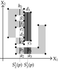
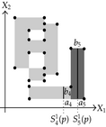
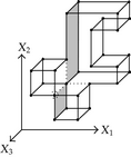
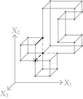
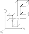
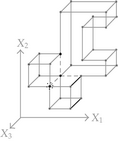
Consider the 3D-OPP p shown in Figure 5. Suppose that the ordering of the coordinates of 3D-EVM of p is X1X2X3. All the vertices of p are extreme except that with a dotted circle, because it has five incident edges and four of them are odd edges, while the fifth one, which is parallel to X3-axis, is, in fact, an even edge; hence, it does not belong to any brink of p. There are another two even edges in p: one of them is parallel to X1-axis while the other to X2-axis. Tables 4 and 5 show the way Algorithm 4 discovers faces, perpendicular to X1-axis, and vertices of p (we recall that our algorithm lists boundary elements’ vertices in the order they are discovered). Table 4 corresponds to the processing of forward differences. is composed by only one component and its 2D-EVM shares the discovering of four vertices. Three of them correspond to projections of extreme vertices of p, because they have only 2 coordinates, while the fourth one precisely corresponds to the projection of the nonextreme vertex indicated in Figure 5. The vertices are completed, in order to have three coordinates, by annexing them the common coordinate of its corresponding forward difference . By this way, vertices v1, v2, v3, and v4, and the face they define, are initially discovered. Via Algorithm 3, is separated in two components. Each component corresponds to a new face defined by four vertices. Both faces and the eight vertices are, respectively, added to the lists of discovered faces and vertices.
| Forward difference | Connected components labeling | Discovered vertices and faces | |
|---|---|---|---|
| v1, v2, v3, v4 | |||
 |
 |
 |
|
 |
 |
 |
|
 |
 |
|
|
 |
 |
 |
|
 |
 |
|
|
| Backward difference | Connected components labeling | Discovered vertices and faces | |
|---|---|---|---|
 |
 |
 |
|
 |
 |
 |
|
 |
|
||

Table 5 shows the processing of backward differences. corresponds to a 2D-OPP in which six of its seven vertices are extreme vertices. When applying Algorithm 3 over , we obtained two components. The extreme vertices of are present in the components, but a new vertex appear which is product of the separation of the original face. Such a vertex (v2), in fact, was previously identified when processing (Table 4). nonextreme vertex v1 is present in the second component: it was also identified when was processed. The remaining vertices in both components, and the faces they define, are appended to their corresponding lists.
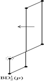
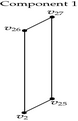
Each one of the 2D components in the forward and backward differences of p is used as input for the recursive calls of Algorithm 4. These calls have the objective of identifying edges perpendicular to X2-axis. Table 6 presents the way Algorithm 4 discovers of some of these edges. When is sent as input its corresponding 1D forward and backward differences, perpendicular to X2-axis, are computed. Two edges are identified: one is defined by vertices v3 and v4 (an odd edge), while the other is defined by vertices v1 and v2. Edge {v1, v2} is one of the three even edges that 3D-OPP p has. According to previous sections, nonextreme vertices are ignored by the EVM. Moreover, when brinks are obtained from an EVM, even edges remain unidentified, because they are not part of brinks. Tables 4 and 6 exemplify situations where these types of former boundary elements are obtained after computing forward and backward differences.
| Input 2D-OPP | 1D Forward and backward differences | Connected components labeling | Discovered edges | |
|---|---|---|---|---|
 |
 |
 |
 |
|
 |
 |
|
||
 |
 |
 |
 |
|
 |
 |
|
||
 |
 |
 |
 |
|
 |
 |
|
||
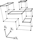
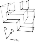
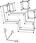
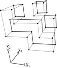
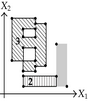
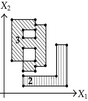
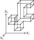
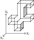
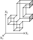
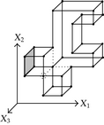
When considering nD orthogonal polytopes, n ≥ 4, Algorithm 4 is clearly capable of identifying nonextreme vertices and even edges. Furthermore, it is capable of discovering those kD boundary elements that cannot be described via brinks. Consider the 4D-OPP p presented in Figure 6(a). Such polytope can be seen as two hypercubes sharing a face (which is shaded in gray). The face is composed by four nonextreme vertices and four even edges. When p’s brinks, parallel to X1 to X4-axes, are obtained (Figure 6(b)), the shared face’s elements are not present, because the 4D-EVM only stores extreme vertices which in time define brinks which are formed only by odd edges. Figure 6(c) presents the three 3D couplets, perpendicular to X1-axis, of p. Each couplet is formed by a volume. The three volumes appear to intersect, but this is an effect of the 4D-3D-2D projections used. Figure 6(d) presents p’s two 3D forward differences perpendicular to X1-axis. When processing , Algorithm 4 detects a 3D boundary volume defined by eight vertices: four of them correspond to extreme vertices of p, while the other four correspond to the vertices of the shared face: such vertices did not belong to EVM4(p). These four vertices are detected again when processing backward difference (see Figure 6(e)). Three-dimensional forward difference is used, in a recursive call, as input for Algorithm 4 (see Figure 6(f)). When its 2D forward and backward differences, perpendicular to X4-axis, are processed and specifically when processing its only backward difference, the shared face is formerly discovered and stored in the list of p’s boundary faces. The edges of such face are formerly discovered when this face is then sent as input, in a new recursive call, of Algorithm 4.


We conclude this section by mentioning that it is important to take into account the coordinates ordering in an EVM determines which boundary elements are identified. Suppose that we use the sorting X1X4X2X3. Algorithm 2 will extract forward and backward differences perpendicular to X1-axis. Then, in turn, Algorithm 4 shares to identify 3D boundary volumes perpendicular precisely to X1-axis (see Figures 6(d) and 6(e)). When each one of these volumes is sent as input in the corresponding recursive calls, we have input 3D-EVMs sorted as X4X2X3. Hence, there are identified, again, because of the use of Algorithm 2, faces perpendicular to X4-axis. In this phase, we are working with volumes embedded in a 3D space, because of the use of projection operator which has removed the X1-coordinate. But, when the source 4D Space is taken into account, it can be determined, in fact, such faces are perpendicular to the plane described by X1 and X4 axes, because they precisely belong to volumes perpendicular to X1-axis (see Figure 6(f)). When each face, expressed as a 2D-EVM, is sent again as input, we identify edges perpendicular to X2-axis, formally, edges perpendicular to the 3D hyperplane described by X1, X4, and X2 axes. Some applications could require to have access to boundary elements which cannot be identified via a given coordinates ordering. In this sense, a new sorting of the corresponding EVM is required, but it can be achieved in efficient time respect to the number of extreme vertices in the corresponding EVM. By this way, for example, coordinates sorting X3X4X1X2 will share to identify 3D volumes perpendicular to X3-axis, faces perpendicular to the plane X3X4, and edges perpendicular to the 3D hyperplane X3X4X1.
6. An Experimental Time Complexity Analysis for Boundary Extraction under the nD-EVM
- (i)
The units for the time measures are given in nanoseconds.
- (ii)
The evaluations were performed with a CPU Intel Core Duo (2.40 GHz) and 2 Gigabytes in RAM.
- (iii)
Our algorithms were implemented using the Java Programming Language under the Software Development Kit 1.6.0.
- (iv)
Our testing consider n = 2,3, 4,5.
- (v)
For each n, we have generated 10,000 random nD-OPPs. Each generated nD-OPP g was, respectively, expressed as EVMn(g) and sent as input to Algorithm 4.
- (vi)
In the 2D, 3D, 4D, and 5D cases, the considered coordinates ordering were X1X2, X1X2X3, X1X2X3X4, and X1X2X3X4X5, respectively. This implies that, as specified in Section 5, we identified first (n − 1)D boundary elements perpendicular to X1-axis, then we identified (n − 2)D boundary elements perpendicular to X2-axis, and so on.
- (vii)
Once the generation of nD-OPPs has finished and the algorithm was evaluated, we proceed with a statistical analysis in order to find a trendline of the form t = axb, where x = Card (EVMn(g)), that fits as good as possible to our measures in order to provide an estimation of the temporal complexity of Algorithm 4 for each value of n. The quality of the approximation curve is assured by computing the coefficient of determination R2.
Table 7 shows some statistics related to our generated polytopes. In Figure 7 the behavior of Algorithm 4 with our testing sets of nD-OPPs can be visualized. In the same chart the corresponding trendline for each value of n whose associated equations are shown in Table 8 can be also appreciated.
| n | Max card (EVMn(g)) |
Min card (EVMn(g)) |
Median card (EVMn(g)) |
Average card (EVMn(g)) |
Standard deviation card (EVMn(g)) |
|---|---|---|---|---|---|
| 2 | 7,016 | 4 | 3,682 | 3,633.35 | 2,004.88 |
| 3 | 6,742 | 0 | 5,334 | 4,695.53 | 1,772.10 |
| 4 | 6,830 | 0 | 5,362 | 4,727.48 | 1,781.45 |
| 5 | 7,310 | 0 | 5,392 | 4,825.45 | 1,876.69 |
| n | Trendline t = axb | a | b | R2 |
|---|---|---|---|---|
| 2 | t = 484.02x1.4313 | 484.02 | 1.4313 | 0.9866 |
| 3 | t = 27,391x1.1214 | 27,391 | 1.1214 | 0.9962 |
| 4 | t = 33,300x1.1744 | 33,300 | 1.1744 | 0.9835 |
| 5 | t = 34,957x1.2047 | 34,957 | 1.2047 | 0.9658 |

We can then observe in the obtained trendlines (Table 8) that the exponents associated with the number of vertices vary between 1 and 1.5. These experimentally identified complexities for our Algorithm 4 provide us elements to determine its temporal efficiency when we extract boundary elements from an nD-OPP expressed as an EVM.
7. Concluding Remarks and Future Work
In this work, we have provided two contributions: an algorithm for computing connected components labeling and an algorithm for extracting boundary elements. The procedures deal with the dominion of the n-dimensional orthogonal pseudo-polytopes, and they are specified in terms of the extreme vertices model in the n-dimensional space. As seen before, both algorithms are sustained in the basic methodologies provided by the nD-EVM. As commented in Section 2, some of such basic algorithms in time are sustained in the MergeXor algorithm. It computes the regularized XOR between two nD-OPPs expressed in the EVM but in terms of the ordinary XOR operation. This implies MergeXor, as its name indicates, is implemented as a merging procedure that only takes in account those extreme vertices present in the first or second input EVMs but not in both. Therefore, it can be specified as a merging-like procedure with an execution linear time given by the sum of the cardinalities of the input EVMs [1]. On one hand, this has as a consequence the temporal efficiency of the basic EVM algorithms. On the other hand, as seen in Section 6 and from an empirical point of view, we have elements to sustain the efficiency of the algorithms provided here.
As part of our future work, and particularly, immediate applications for Algorithms 3 and 4, we comment that we will attack the problem related to the automatic classification of video sequences. In [23], we describe a methodology for representing 2D color video sequences as 4D-OPPs embedded in a 4D color-space-time geometry. Our idea is the use of geometrical and topological properties, such as boundary descriptions, connected components, and discrete compactness, in order to determine similarities and differences between sequences and for instance to classify them. In [5], part of this work has been boarded using only discrete compactness, and the obtained results are promising. We are going to incorporate the information provided by Algorithms 3 and 4 in order to determine if they can contribute to enhance the results.

