Estimation of Failure Probability and Its Applications in Lifetime Data Analysis
Abstract
Since Lindley and Smith introduced the idea of hierarchical prior distribution, some results have been obtained on hierarchical Bayesian method to deal with lifetime data. But all those results obtained by means of hierarchical Bayesian methods involve complicated integration compute. Though some computing methods such as Markov Chain Monte Carlo (MCMC) are available, doing integration is still very inconvenient for practical problems. This paper introduces a new method, named E-Bayesian estimation method, to estimate failure probability. In the case of one hyperparameter, the definition of E-Bayesian estimation of the failure probability is provided; moreover, the formulas of E-Bayesian estimation and hierarchical Bayesian estimation and the property of E-Bayesian estimation of the failure probability are also provided. Finally, calculation on practical problems shows that the provided method is feasible and easy to perform.
1. Introduction
In the area related to the reliability of industrial products, engineers often deal with the truncated data in life testing of products, where the data sometimes have small sample size or have been censored, and the products of interest have high reliability. In the literature, Lindley and Smith [1] first introduced the idea of hierarchical prior distribution. Han [2] developed some methods to construct hierarchical prior distribution. Recently, hierarchical Bayesian methods have been applied to data analysis [3]. However, complicated integration compute is a hard work by using hierarchical Bayesian methods in practical problems, though some computing methods such as Markov Chain Monte Carlo (MCMC) methods are available [4, 5].
Han [6] introduced a new method—E-Bayesian estimation method—to estimate failure probability in the case of two hyperparameters, proposed the definition of E-Bayesian of failure probability, and provided formulas for E-Bayesian estimation of the failure probability under the cases of three different prior distributions of hyperparameters. But we did not provide formulas for hierarchical Bayesian estimation of the failure probability nor discuss the relations between the two estimations. In this paper, we will introduce the definition for E-Bayesian estimation of the failure probability, provide formulas both for E-Bayesian estimation and hierarchical Bayesian estimation, and also discuss the relations between the two estimations in the case of only one hyperparameter. We will see that the E-Bayesian estimation method is really simple.
Conduct type I censored life testing m time, denote the censored times as ti (i = 1,2, …, m), the corresponding sample numbers as ni, and the corresponding failure sample numbers observed in the testing process as ri (ri = 0,1, 2, …, ni).
In the situation where no information about the life distribution of tested products is available, Mao and Luo [7] introduce a so-called curves fitting distribution method to give the estimation of the failure probability pi at time ti, pi = P(T < ti) for i = 1,2, …, m, where T is the life of a product.
This paper introduces a new method, called E-Bayesian estimation method, to estimate failure probability. The definition and formulas of E-Bayesian estimation of the failure probability are described in Sections 2 and 3, respectively. In Section 4, formulas of hierarchical Bayesian estimation of the failure probability are proposed. In Section 5, the properties of E-Bayesian estimation are discussed. In Section 6, an application example introduces given. Section 7 is the conclusions.
2. Definition of E-Bayesian Estimation of pi
According to Han [2], a and b should be chosen to guarantee that π(pi∣a, b) is a decreasing function of pi. Thus 0 < a < 1, b > 1.
Given 0 < a < 1, the larger the value of b, the thinner the tail of the density function. Berger had shown in [8] that the thinner tailed prior distribution often reduces the robustness of the Bayesian estimate. Consequently, the hyperparameter b should be chosen under the restriction 1 < b < c, where c is a given upper bound. How to determine the constant c would be described later in an example.
Since a ∈ (0,1) and 1/2 is an expectation of uniform on (0, 1), that we take a = 1/2. When 1 < b < c and a = 1/2, π(pi∣a, b) also is a decreasing function of pi.
The definition of E-Bayesian estimation was originally addressed by Han [6] in the case of two hyperparameters. In the case of one hyperparameter, the E-Bayesian estimation of failure probability is defined as follows.
Definition 1. With being continuous,
3. E-Bayesian Estimation of pi
Theorem 2. For the testing data set {(ni, ri, ti), i = 1, …, m} with type I censor, where ri = 0,1, 2, …, ni, let and . If the prior density function π(pi∣b) of pi is given by (3), then, we have the following.
- (i)
With the quadratic loss function, the Bayesian estimation of pi is
() - (ii)
If prior distribution of b is uniform on (1, c), then E-Bayesian estimation of pi is
()
Proof. (i) For the testing data set {(ni, ri, ti), i = 1, …, m} with type I censor, where ri = 0,1, 2, …, ni, according to Han [6], the likelihood function of samples is
Combined with the prior density function π(pi∣b) of pi given by (3), the Bayesian theorem leads to the posterior density function of pi,
Thus, with the quadratic loss function, the Bayesian estimation of pi is
(ii) If prior distribution of b is uniform on (1, c), then, by Definition 1, the E-Bayesian estimation of pi is
This concludes the proof of Theorem 2.
4. Hierarchical Bayesian Estimation
If the prior density function π(pi∣b) of pi is given by (3), how can the value of hyperparameter a be determined? Lindley and Smith [1] addressed an idea of hierarchical prior distribution, which suggested that one prior distribution may be adapted to the hyperparameters while the prior distribution includes hyperparameters.
Theorem 3. For the testing data set {(ni, ri, ti), i = 1, …, m} with type I censor, where ri = 0,1, 2, …, ni, let and . If the hierarchical prior density function π(pi) of pi is given by (12), then, using the quadratic loss function, the hierarchical Bayesian estimation of pi is
Proof. According to the course of the proof of Theorem 2, the likelihood function of samples is
From the hierarchical prior density function of pi given by (12), the Bayesian theorem leads to the hierarchical posterior density function of pi,
With the quadratic loss function, the hierarchical Bayesian estimation of pi is
Thus, the proof is completed.
5. Property of E-Bayesian Estimation of pi
Now we discuss the relations between and in Theorems 2 and 3.
Proof. According to the course of the proof of Theorem 2, we have that
When b ∈ (1, c), (ei + (1/2)/si + b + (1/2)) is continuous; by the mean value theorem for definite integrals, there is at least one number b1 ∈ (1, c) such that
According to (17) and (18), we have that
According to the relations of Beta function and Gamma function, we have that
When b ∈ (1, c), we have that B(ei + (1/2), si + b − ei) > 0, and (ei + (1/2)/si + b + (1/2)) is continuous; by the generalized mean value theorem for definite integrals, there is at least one number b2 ∈ (1, c) such that
According to Theorem 3, we have that
According to (19) and (22), we have that .
Thus, the proof is completed.
Theorem 4 shows that and are asymptotically equivalent to each other as si tends to infinity. In application, and are close to each other, when si is sufficiently large.
6. Application Example
Han [6] provided a testing data of type I censored life testing for a type of engine, which is listed in Table 1 (time unit: hour).
| i | 1 | 2 | 3 | 4 | 5 | 6 | 7 | 8 | 9 |
|---|---|---|---|---|---|---|---|---|---|
| ti | 250 | 450 | 650 | 850 | 1050 | 1250 | 1450 | 1650 | 1850 |
| ni | 3 | 3 | 3 | 3 | 4 | 4 | 4 | 4 | 4 |
| ri | 0 | 0 | 0 | 0 | 0 | 1 | 0 | 1 | 1 |
| ei | 0 | 0 | 0 | 0 | 0 | 1 | 1 | 2 | 3 |
| si | 32 | 29 | 26 | 23 | 20 | 16 | 12 | 8 | 4 |
By Theorems 2, 3, and Table 1, we can obtain , , and . Some numerical results are listed in Table 2.
| c | 2 | 3 | 4 | 5 | 6 | Range |
|---|---|---|---|---|---|---|
| 0.014707 | 0.014497 | 0.014294 | 0.014099 | 0.013911 | 0.000796 | |
| 0.014693 | 0.014458 | 0.014228 | 0.014004 | 0.013788 | 0.000905 | |
| 0.000014 | 0.000039 | 0.000066 | 0.000095 | 0.000123 | 0.000109 | |
| 0.016130 | 0.015878 | 0.015636 | 0.015404 | 0.015181 | 0.000949 | |
| 0.016114 | 0.015832 | 0.015557 | 0.015291 | 0.015035 | 0.001079 | |
| 0.000016 | 0.000046 | 0.000079 | 0.000113 | 0.000146 | 0.000130 | |
| 0.017859 | 0.017551 | 0.017256 | 0.016975 | 0.016705 | 0.001154 | |
| 0.017839 | 0.017495 | 0.017160 | 0.016838 | 0.016530 | 0.001309 | |
| 0.000020 | 0.000056 | 0.000096 | 0.000137 | 0.000175 | 0.000155 | |
| 0.020002 | 0.019618 | 0.019252 | 0.018904 | 0.018572 | 0.001430 | |
| 0.019978 | 0.019548 | 0.019133 | 0.018736 | 0.018358 | 0.001620 | |
| 0.000024 | 0.000070 | 0.000119 | 0.000168 | 0.000214 | 0.000190 | |
| 0.022731 | 0.022237 | 0.021770 | 0.021328 | 0.020909 | 0.001822 | |
| 0.022699 | 0.022148 | 0.021619 | 0.021118 | 0.020642 | 0.001620 | |
| 0.000032 | 0.000089 | 0.000151 | 0.000210 | 0.000267 | 0.000235 | |
| 0.083355 | 0.081160 | 0.079112 | 0.077194 | 0.075394 | 0.007961 | |
| 0.083237 | 0.080856 | 0.078634 | 0.076573 | 0.074661 | 0.008576 | |
| 0.000118 | 0.000304 | 0.000478 | 0.000621 | 0.000733 | 0.000615 | |
| 0.107188 | 0.103613 | 0.100335 | 0.097317 | 0.094524 | 0.012664 | |
| 0.107011 | 0.103177 | 0.099683 | 0.096509 | 0.093620 | 0.013391 | |
| 0.000177 | 0.000436 | 0.000652 | 0.000808 | 0.000904 | 0.000727 | |
| 0.250209 | 0.238819 | 0.228697 | 0.219623 | 0.211428 | 0.030781 | |
| 0.250016 | 0.238721 | 0.229136 | 0.220951 | 0.213898 | 0.036118 | |
| 0.000193 | 0.000099 | 0.000439 | 0.000672 | 0.002470 | 0.002277 | |
| 0.584689 | 0.542771 | 0.507871 | 0.478226 | 0.452640 | 0.132050 | |
| 0.589643 | 0.559105 | 0.528191 | 0.523250 | 0.512187 | 0.077456 | |
| 0.004954 | 0.016334 | 0.020320 | 0.045024 | 0.059547 | 0.054594 | |
From Table 2, we find that for some c (c = 2,3, 4,5, 6), , and are very close to each other and satisfy Theorem 4; for different c (c = 2,3, 4,5, 6), and are all robust (when i = 9, there exists some difference). In application, the author suggests selecting a value of c in the middle point of interval [2, 6], that is, c = 4.
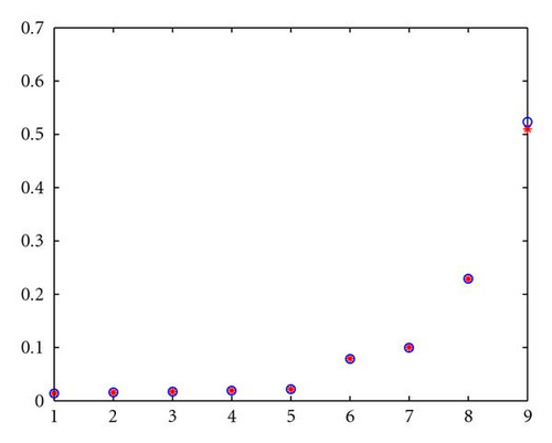
When c = 4, some numerical results are listed in Table 3 and Figure 1.
| i | 1 | 2 | 3 | 4 | 5 |
|---|---|---|---|---|---|
| 0.014294 | 0.015636 | 0.017256 | 0.019252 | 0.021770 | |
| 0.014228 | 0.015557 | 0.017160 | 0.019133 | 0.021619 | |
| 0.000066 | 0.000079 | 0.000096 | 0.000119 | 0.000151 | |
| i | 6 | 7 | 8 | 9 | |
| 0.079112 | 0.100335 | 0.228697 | 0.507871 | ||
| 0.078634 | 0.099683 | 0.229136 | 0.528191 | ||
| 0.000478 | 0.000652 | 0.000439 | 0.020320 | ||

Range: in Figure 1, * is the results of and o is the results of .
From Table 3 and Figure 1, we find that and are very close to each other and consistent with Theorem 4.
From Table 3, we find that the results of and are very close to the corresponding results of Han [6].
From (24) and Table 3, we can obtain and . Some numerical results of and are listed in Table 4.
| Parameter estimate | ||
|---|---|---|
| E-Bayesian estimate | 2.640846864 | 2738.461813 |
| Hierarchical Bayesian estimate | 2.678276374 | 2639.899868 |
| Difference between the above two estimates | 0.037429506 | 98.56194500 |
From Table 4, we find that the results of and are very close to the corresponding results of Han [6].
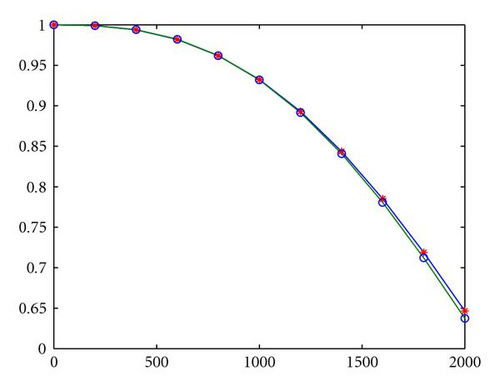
From (25) and Table 4, we can obtain the estimate of the reliability with some numerical results of and listed in Table 5 and Figure 2.
| t | 200 | 600 | 1000 | 1400 | 1800 | 2000 |
|---|---|---|---|---|---|---|
| 0.999003 | 0.982019 | 0.932467 | 0.843643 | 0.718796 | 0.646553 | |
| 0.999056 | 0.982247 | 0.932059 | 0.840921 | 0.712032 | 0.637398 | |
| 0.000053 | 0.000228 | 0.000408 | 0.002722 | 0.006764 | 0.009155 |

Note that is the estimate of reliability at moment t with regard to , is the estimate of reliability at moment t with regard to , and .
Range: in Figure 2, * is the results of and o is the results of .
From Table 5, we find that when t = 200,600,1000,1400, 1800,2000, and the results of and are very close to those of Han [6].
7. Conclusions
This paper introduces a new method, called E-Bayesian estimation, to estimate failure probability. The author would like to put forward the following two questions for any new parameter estimation method: (1) how much dependence is there between the new method and the other already-made ones? (2) In which aspects is the new method superior to the old ones?
For the E-Bayesian estimation method, Theorem 4 has given a good answer to the above question (1) and, in addition, the application example shows that and satisfy Theorem 4.
To question (2), from Theorems 2 and 3, we find that the expression of the E-Bayesian estimation is much simple, whereas the expression of the hierarchical Bayesian estimation relies on beta function and complicated integrals expression, which is often not easy.
Reviewing the application example, we find that the E-Bayesian estimation method is both efficient and easy to operate.
Acknowledgments
The author wish to thank Professor Xizhi Wu, who has checked the paper and given the author very helpful suggestions. This work was supported partly by the Fujian Province Natural Science Foundation (2009J01001), China.


