Volume 2011, Issue 1 325690

Research Article

Open Access

Modeling and Analysis of Material Flows in Re-Entrant Supply Chain Networks Using Modified Partial Differential Equations

Fenglan He

Department of Industrial Engineering, School of Mechanical Engineering, Shanghai Jiao Tong University, 800 Dongchuan Road, Shanghai 200240, China sjtu.edu.cn

Search for more papers by this author

Ming Dong,

Corresponding Author

Ming Dong

[email protected]

Department of Operations Management, Antai College of Economics & Management, Shanghai Jiao Tong University, 535 Fahua Zhen Road, Shanghai 200052, China sjtu.edu.cn

Search for more papers by this author

Xiaofeng Shao,

Xiaofeng Shao

Department of Operations Management, Antai College of Economics & Management, Shanghai Jiao Tong University, 535 Fahua Zhen Road, Shanghai 200052, China sjtu.edu.cn

Search for more papers by this author

Fenglan He,

Fenglan He

Department of Industrial Engineering, School of Mechanical Engineering, Shanghai Jiao Tong University, 800 Dongchuan Road, Shanghai 200240, China sjtu.edu.cn

Search for more papers by this author

Ming Dong,

Corresponding Author

Ming Dong

[email protected]

Department of Operations Management, Antai College of Economics & Management, Shanghai Jiao Tong University, 535 Fahua Zhen Road, Shanghai 200052, China sjtu.edu.cn

Search for more papers by this author

Xiaofeng Shao,

Xiaofeng Shao

Department of Operations Management, Antai College of Economics & Management, Shanghai Jiao Tong University, 535 Fahua Zhen Road, Shanghai 200052, China sjtu.edu.cn

Search for more papers by this author

First published: 07 February 2011

https://doi.org/10.1155/2011/325690

Citations: 1

Academic Editor: Shuyu Sun

Share a link

Email
Wechat
Bluesky

Abstract

The basic partial differential equation (PDE) models for supply chain networks with re-entrant nodes and their macroscopic are proposed. However, through numerical examples, the basic continuum models do not perform well for multiple re-entrant systems. Then, a new state equation considering the re-entrant degree of the products is introduced to improve the effectiveness of the basic continuum models. The applicability of the modified continuum models for re-entrant supply chains is illustrated through numerical examples. Finally, based on the modified continuum model, numerical examples of different re-entrant degrees are given, meanwhile, the changes in the WIP and outflux are analyzed in details for multiple re-entrant supply chain systems.

1. Introduction

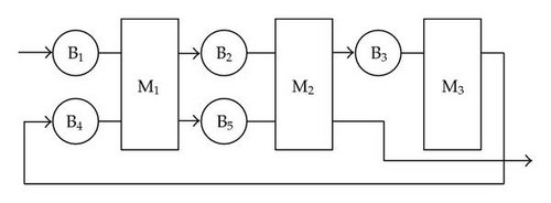
In recent years, factories and production systems have become larger and more complicated. The re-entrant manufacturing system is a typical example, which indicates that work in process (WIP) repeatedly passes through the same workstation at different stages of the process routes. Figure 1 gives a simplified model of re-entrant systems. The model consists of three workstations and five buffers; the arrows in the figure indicate the processing path of a lot. From Figure 1, it can be seen that the lot passes through the same workstations M₁ and M₂ twice, which is a typical situation of a re-entrant system. A re-entrant supply chain network consists of many such manufacturing systems. Understanding the behavior of large supply chains under different policies and scenarios is a major issue for many businesses today. In large factories, no experiments can be done involving whole supply chains. Therefore, simulation models are developed, which substitute for the real environment. There are several methods to model the multiple re-entrant production flows: Petrinet, queuing network, fluid network, and partial differential equation (PDE).

Details are in the caption following the image — **Figure 1**
Open in figure viewer PowerPoint

A simplified model for a re-entrant system.

Petrinet is a mathematical tool to describe and analyze the logical relations of state changes for discrete event dynamic systems. It has been widely used in modeling, simulating, analyzing, and controlling of the discrete event dynamic systems. Compared with some other description tools, Petrinet model is especially easy to describe concurrent phenomena and simulate the parallel systems. On account of directly describing production processes, Petrinet model has been used to model the re-entrant manufacturing systems. However, it is extremely hard to solve the analytic solutions with the increase of system complexity. Wang and Wu [1] put forward an object-oriented hybrid Petrinet model of semiconductor manufacturing lines. Lin et al. [2] established a model of the re-entrant semiconductor production lines using Petrinets and studied on the stability of the system using buffer-boundless approach. Dong and Chen [3] developed a modular modeling approach based on object-oriented predicate/transition nets (OPTNs) for the analysis of supply chain process models.

Queuing network model treats each workstation as an individual discrete queue, then these independent queues are connected to form queuing networks according to the production flow. Queuing network model can directly describe the process of production lines and supply chain networks. A methodology for supply chain inventory analysis and optimization was presented by linking production authorization (PA) strategy to queueing models [4]. The statistics of arrival flow of the fluid model in queuing systems has been studied [5, 6]. Dong and Chen [7] proposed a network of inventory-queue models for the performance modeling and analysis of an integrated supply chain network. S. Kumar and P. R. Kumar [8] focused on the analysis of queuing theory of the re-entrant manufacturing systems. However, the analytic solution could be obtained only for the small-size systems based on the queuing models. When the scale of production systems or supply chain networks become large, the number of system states would grow exponentially and a combinatorial explosion problem would occur. Therefore, the queuing models have some difficulties in analysis of the real large-scale re-entrant supply chain networks. Most of the queuing models can only be used to evaluate the stability of some scheduling policies and difficult to be used directly for the real-world supply chains.

Since most supply chains deal with individual parts and the processes that those parts undergo, the above two discrete event models can describe a lot of details of the studied system. While discrete event simulators have been highly successful to simulate single factories, they are computationally too expensive to simulate even a moderately complicated supply chains. Meanwhile, they are not scalable to a full supply chain. Therefore, a new modeling method called approximate modeling appears.

There are two kinds of approximate models: one is the so-called fluid model. It comes from traffic theory and was introduced by Newell [9] to approximately solve queuing problems. It treats the queue length l(t) as a continuous variable. The change rate of a queue length is equal to the arrival rate λ(t) minus the processing rate μ(t) when the queue length is not 0, otherwise the change rate of a queue length is 0. Hence, fluid models can quickly obtain the results by solving the ordinary differential equations. The time required for computing is not affected with the increase of material flows. The fluid models can be used not only to optimize the control system but also to reflect the long-term performance behavior of the system in the dynamic states.

However, one of the most important shortcomings of fluid models is that they cannot reflect the stochasticity of the production processes very well, that is, in the above equation, if λ(t) and μ(t) are mean rates, then this is a fully deterministic system, stochasticity is not modeled at all. Otherwise, if λ(t) and μ(t) are stochastic processes, then some theoretical analysis will be allowed. But this will degrade the advantages of a continuum models as a simulation tool [10].

Dai and Weiss [11] analyzed the relationship between the stability of the fluid model and the stability of the scheduling policies for the related queuing networks. Here, the stability of the fluid models is expressed by the boundedness of the fluid variables for a fixed influx. Göttlich [12] deduced the conservation laws under the form of ordinary differential and proved the existence of its solution based on the fluid models of supply chain networks.

The other approximate model is called partial differential equation (PDE) model. PDE models are actually continuum limit of fluid models. PDE models do have several advantages, that is, they are scalable; more detailed results can be found as compared to fluid models, and more importantly, they are amenable to optimization and control [13].

Recently, the continuous models have been applied to many fields and have achieved some significant research results. Anderson [14] established the basic continuous model for supply chains and described production flow of the system using rate equations macroscopically. Lee et al. [15] studied the supply chain simulation with combined discrete-continuous modeling method. It integrates the wide applicability of the discrete event simulation (DES) and fast computation of the continuum models together. Armburster et al. [16] introduced the concept of materials’ density and established the continuous model of large-scale re-entrant manufacturing systems and proposed new state equations so that the continuous model could be used to the real production systems. Compared with a DES model, van den Berg et al. [17] verified the validity of the continuous model of simple serial production systems and then solved the optimal control problems with consideration of the demand growth. Unver et al. [18] presented a continuum (traffic flow like) model for the flow of products through complex production networks, based on statistical information obtained from extensive observations of the system. The resulting model consists of a system of hyperbolic conservation laws, which exhibit the correct diffusive properties given by the variance of the observed data.

In this paper, in order to accurately describe the multiple re-entrant supply chain networks from macroscopic perspective, a modified model is proposed, which can reflect how the re-entrant degree of a product impacts the system performance. Based on the queuing theory, we restrict our attention on establishing a new state equation considering the re-entrant degrees of jobs or products, meanwhile, we will also verify the validity of the modified PDE model for multiple re-entrant semiconductor supply chain systems by a numerical experiment. And finally, the changes of the WIP and outflux in the case of different re-entrant factors are analyzed based on the modified PDE model.

The structure of this paper is organized as follows: in Section 2, the basic continuum model is presented and a numerical experiment is carried out to verify the validity of the basic model. Section 3 introduces the concept of re-entrant factor to improve the basic continuum model and verifies its effectiveness through an example. In Section 4, based on the modified continuous model, the WIP profile and outflux are analyzed in the case of different re-entrant factors. Finally, some conclusions are given in Section 5.

2. The Basic Continuum Model

2.1. Basic Model

Recently, continuum models for large-scale multiple re-entrant production systems have become an important research topic. Such a description is appropriate for a semiconductor manufacturing fab involving a large number of items in many stages. As ρ(x, t) is the conserved variable, it is the density of the products with units [units/space] in the system. Here, x denotes the completion variable, x = 0 describes raw products that have just entered into the factory, and x = 1 denotes finished products that are ready to exit from the system. So, in the closed interval x ∈ [0,1]. The total number of products in the system can be found by taking the integral of density ρ(x, t) of products over the stage variable x from 0 to 1. Therefore, the total WIP W(t) as a function of time can be obtained as follows:

()

According to the conservation law, assuming that there is a unique entry and exit for the system and the yield is 100%, PDE models can be given by

()

where v(ρ(x, t)) is a velocity function that depends on the density ρ(x, t) only. For a re-entrant supply chain system, we assume that v(ρ(x, t)) can be described by a state equation of the following form:

()

Here, v₀ is the velocity for the empty supply chain system and W_max is the maximal load (capacity of the supply chain system). Clearly, the velocity v(ρ(x, t)) is determined by the total WIP. The boundary condition for the start rate λ(t) of products entering the supply chain system at x = 0 is then defined as

()

An arbitrary initial condition for the density of the products can be expressed as

()

The production process in the supply chain network is described as an equivalent M/M/1 queue. The state variable ρ_eq denotes the equilibrium density of the supply chain system as a whole. Let ρ = ρ_eq, then ρ(0, t) = ρ_eq and v = v_eq = 1/τ. Correspondingly, the associated cycle time in steady state is τ = 1/v_eq. Since a job arriving at a queue with a processing rate is μ = 1/v_max, the cycle time τ = μ(1 + L) can be obtained according to the queuing theory; therefore, the equilibrium velocity becomes

()

Equation (2.6) is a widely used expression between v and ρ for large-scale multiple re-entrant supply chain systems; note that the velocity v only depends upon the WIP at stage x. Therefore, Equation (2.2) can be rewritten as

()

Hence, assuming an initial WIP distribution ρ₀(x) in the factory is given, the resulting full PDE model for the single-product multiple re-entrant supply chain systems is given as follows

()

If the influx λ(t) and the initial condition ρ₀(x) are nonnegative, then the density will remain nonnegative. We use an upwind scheme [19] to discretize the PDE which is given by the following equation:

()

where i = 1,2, …, N, and j = 0,1, …, M − 1. Δt and Δx are the step sizes in time and space, respectively. Based on the boundary condition, the propagation scheme is given by

()

Since the Courant-Friedrich-Levy (CFL) condition is necessary for stability, the time step Δt and the space step Δx must satisfy the formulation as follows: |(Δt/Δx)v_max(t)| ≤ 1. Here, v_max(t) is the maximum of all occurring velocities in the system at time t.

Based on the above formula, the density distribution of each moment ρ(x_i, t_j) can be obtained. Therefore, the system throughput rate q(x_N, t_j) of each moment can also be computed as follows:

()

Furthermore, the total WIP

can be obtained via the extended Simpson’s rule quadrature, then the following equation can be obtained:

()

Finally, the density distribution ρ(x_i, t_j) and throughput q(x_N, t_j) of each moment can be obtained.

2.2. Numerical Experiments

Mini-Fab is a simplified model of the semiconductor production line, which has all the important features of the re-entrant semiconductor manufacturing systems, such as re-entrant, different processing time, and batch production. Currently, many scholars have done a lot of research work based on the Mini-Fab. The Mini-Fab contains 5 machines grouped into 3 tool sets; the product comprises of 6 processing steps, each tool set is visited twice, which is shown in Figure 2 [20].

For convenience, we make the following basic assumptions on the model:

(1)
the product yield rate is 100%, namely, there is no rework problem;
(2)
the system is a continuous production process for 24 hours a day;
(3)
the system does not take into account the time of carrying, loading and discharging, adjusting equipment, and premaintaining equipment and downtime.

Now it is assumed that there is one product D in the Mini-Fab, processing steps and processing time shown in Table 1.

Table 1. Processing time of the product D at each step.

Machining centers	Processing time (hours)
Machines A & B	Step 1: 1.5	Step 5: 1.5
Machines C & D	Step 2: 0.5	Step 4: 1
Machine E	Step 3: 1	Step 6: 0.5

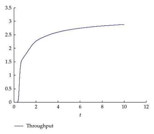
Based on the basic continuous model, the parameters are assumed as follows: P = 0.25 (days), v_max = 4 (units/day), λ = 5 (units/day). We typically start up with an empty production system; the total running time of the production lines is 10 (days). Let Δt = 0.001 and Δx = 0.01, then Δx and Δt satisfy the CFL stability condition (Δt/Δx)v_max < 1. The system throughput can be obtained through the simulation based on the basic PDE model of (2.8). Figure 3 indicates that the system throughput is about 3.2 (units/day) during the steady state.

Once the throughput of the basic continuous models is obtained, the corresponding Mini-Fab simulation model can be built using simulation package ExtendSim [21] to verify the validity of the models with a period of one year. As can be seen from Figure 4 that the throughput during the steady state is about 5 (units/day) through the ExtendSim simulation.

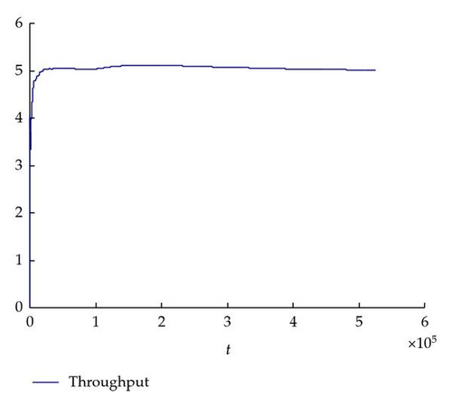
Comparing Figure 3 with Figure 4, it is obviously found that there are some differences between the throughput results of the two models. This is because the basic continuous model of (2.8) is built on the basis of a large number of materials, and many re-entrant steps in the systems and some important characteristics of semiconductor production systems are not captured. Therefore, the further investigation is needed to explore more precise models for multiple re-entrant production systems.

3. The Modified Continuum Model

3.1. Modified Model

It is worth noting that the state equations can reflect the characteristics of systems—any change of the multiple re-entrant production systems may lead to a different state equation. Equation (2.6) is a quite general state equation, in order to capture some important features of multiple re-entrant supply chain systems, so a more specified relationship is required for computing velocities numerically. Lefeber and Armbruster [22] presented a more sophisticated re-entrant factory model through the use of integration kernels. For the general supply chain systems (non-re-entrant systems), Sun and Dong [23] described several kinds of state equations and the corresponding cycle times. Although there are many kinds of continuum models for describing the re-entrant production system currently, they do not reflect how the re-entrant degree of the product impacts the system performance. Hence, a new concept reflecting the re-entrant degree of the products is introduced.

Definition 3.1. Let α be a product re-entrant factor, α equals the ratio of the product processing time of re-entrant steps and the product total processing time.

Re-entrant factor α is the property of product process flows, with the increase of re-entrant factor α, the degree of re-entrant of the product becomes larger and larger. Let P be the total processing time, let P₁ be the re-entrant processing time, and let P₂ be the non-re-entrant processing time. According to the above definition, we can obtain the following formula:

()

In reality, the velocity of products in the system is not only related with the WIP level but also with the re-entrant factor. Let w(t) be the WIP level in the system at a given time t, let w(Δx, t) be the WIP level at interval Δx at time t, let Δx be the interval of the completion of the product, and let Δt be the processing time required to complete the interval Δx. Assume that w(Δx, t) is proportional to Δt and the system consists of two parts: re-entrant processes and non-re-entrant processes, hence, αw(t) is the WIP level of the re-entrant processes at a given time t and also referred to as re-entrant WIP. Similarly, (1 − α)w(t) is the WIP level of non-re-entrant processes at a given time t and also called as non-re-entrant WIP.

According to the queuing theory, the processing cycle time of the re-entrant process τ₁ can be expressed as follows:

()

As for the non-re-entrant processes, assuming the total number of workstations is m, a₁, a₂, …, a_m are the corresponding processing times at each workstation, respectively, and τ₂ is the non-re-entrant processing cycle time, then we have

()

so the total cycle time τ can be written in the following form:

()

Then, the resulting new state equation for the velocity will be given by

()

In order to avoid computational complexity of

, an approximate method is proposed to deal with the non-re-entrant process. Suppose that WIP in non-re-entrant processes follows the uniform distribution in each workstation, then the mean processing time P₂/m and the mean WIP level at each workstation ((1 − α)/m)w(t) can be obtained. According to the queuing theory, the mean cycle time of the non-re-entrant processes at each workstation is [1 + ((1 − α)/m)w(t)](P₂/m), and the total cycle time of the non-re-entrant processes τ₂ is [1 + ((1 − α)/m)w(t)]P₂. Therefore, the total cycle time τ can be expressed as follows:

()

The corresponding new state equation can be obtained as follows:

()

Therefore, the resulting modified whole PDE model is given below:

()

3.2. Validity of the Modified Model

Once the new state equation is obtained, the same example in the previous section can be used to verify the validity of the modified models. According to Figure 2, the total number of workstations is m = 3, the steps 4 to 6 are re-entrant steps. From Table 1, the products’ re-entrant factor α = 0.5 can be easily obtained by definition. Assume that the influx λ is 5 (units/day) and the total running time is 10 (days), the system starts running from an empty state. With Δt = 0.001, Δx = 0.01, then Δx and Δt satisfy the CFL stability condition: v_max · Δt/Δx < 1. Similarly, the modified continuous model (3.8) can be solved via the upwind scheme, and the throughput of the modified models can be obtained, which is plotted in Figure 5.

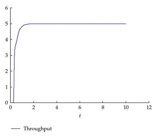
It can be seen that the throughput is initially zero for the re-entrant system. This is due to the time delay and the system initialization (the system starts up with an empty factory), then the system begins to have throughput about 0.25 (days) and increases drastically until the throughput reaches a stable value of 5 (units/day) about 1.5 days. It is obvious that the results are basically consistent with the simulation results obtained from ExtendSim. Therefore, it can be seen that the modified models are more effective for multiple re-entrant supply chain systems.

4. Case Studies for the Different Re-Entrant Factors

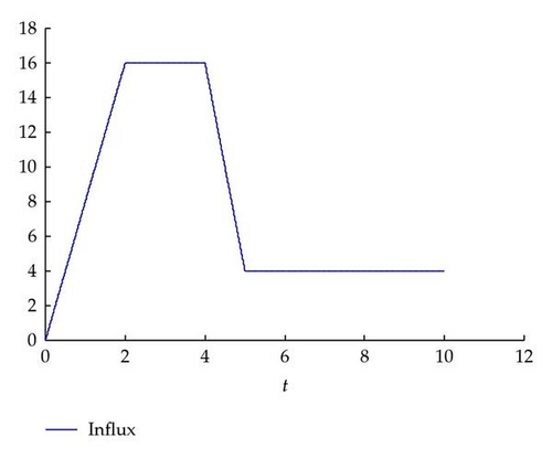
In order to analyze the influence of the re-entrant degree on the WIP profile and outflux for the multiple re-entrant supply chain systems, several scenarios of the different re-entrant factors are presented in this section. Same as the previous section, let v_max = 4 (units/day), a uniform time step size Δt = 0.001 (days), and a uniform spatial interval length Δx = 0.01, then Δx and Δt also satisfy the CFL stability condition (Δt/Δx)v_max < 1. We assume that the varying influx is prescribed first, as shown in Figure 6.

Taking the multiple re-entrant production systems as an example, the system begins to run from an empty factory. We observe the changes of the WIP and outflux in the case of different re-entrant factors. As shown in Figure 7, black and red lines indicate the WIP and outflux, respectively.

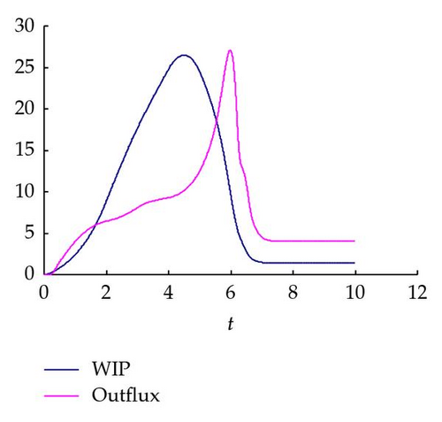
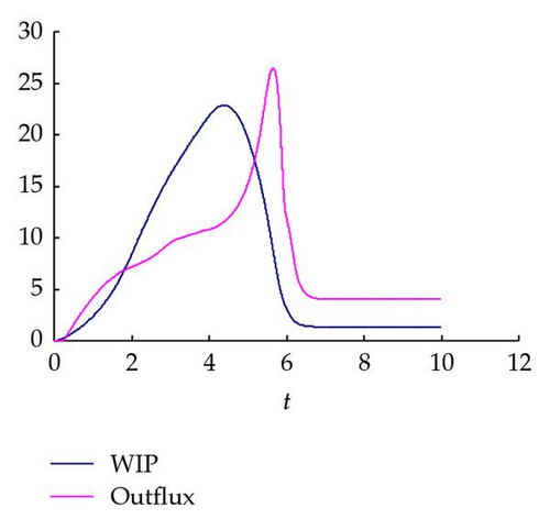
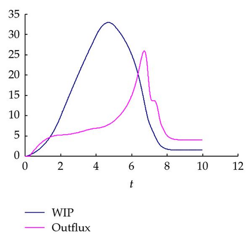
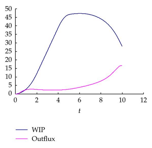
From Figure 7, we can observe that, roughly, the WIP of the modified PDE model shows an increasing trend gradually first to reach the maximum and then it has a decreasing trend until it reaches the stable value. Meanwhile, the outflux of the modified PDE model rises slowly and then sharply reaches the maximum, after that the outflux shows a sudden decrease and then slowly reaches a stable value. Additionally, it is easy to see that the maximum WIP occures a small decrease first and then rises slowly with the increase of the re-entrant factor. Correspondingly, the maximum outflux appears a small increasing trend at first; when the WIP reaches a certain value, the maximum outflux becomes smaller and smaller with the increase of the re-entrant factor. These results are almost consistent with the actual situation; meanwhile, the materials flow can be better controlled according to the WIP profile and outflux.

5. Conclusions

In this paper, the basic continuum models for material flows are first proposed, and its low accuracy for the multiple re-entrant supply chain networks is explained by a numerical experiment. In order to model such systems more precisely, this paper presents a new state equation that takes into account the re-entrant degree of the product. The applicability of the modified continuum model for multiple re-entrant supply chain systems is also illustrated through a numerical example. Afterwards, based on the modified continuum models, some numerical examples on different re-entrant factors are provided, and the impacts of different re-entrant factors on the WIP profile and outflux changes are studied. Meanwhile, some interesting observations are discussed. The proposed model can be used to obtain more accurate results for material flows of the multiple re-entrant supply chain networks from macroscopic perspective.

Acknowledgments

The work presented in this paper has been supported by a Grant from the National High-Tech Research and Development Program (863 Program) of China (no. 2008AA04Z104) and a Grant from National Natural Science Foundation of China (no. 70871077).

References

1 Wang Z. and Wu Q., Object-oriented hybrid PN model of semiconductor manufacturing line, Proceedings of the 4th World Congress on Intelligent Control and Automation, June 2002, 1354–1358, 2-s2.0-0036945876.
Google Scholar
2 Lin C., Xu M., Marinescu D. C., Ren F., and Shan Z., A sufficient condition for instability of buffer priority policies in re-entrant lines, IEEE Transactions on Automatic Control. (2003) 48, no. 7, 1235–1238, 2-s2.0-0042265579, https://doi.org/10.1109/TAC.2003.814268.
10.1109/TAC.2003.814268
Web of Science® Google Scholar
3 Dong M. and Chen F. F., Process modeling and analysis of manufacturing supply chain networks using object-oriented Petri nets, Robotics and Computer-Integrated Manufacturing. (2001) 17, no. 1-2, 121–129, 2-s2.0-0035250688, https://doi.org/10.1016/S0736-5845(00)00045-4.
10.1016/S0736-5845(00)00045-4
Web of Science® Google Scholar
4 Dong M., Inventory planning of supply chains by linking production authorization strategy to queueing models, Production Planning and Control. (2003) 14, no. 6, 533–541, 2-s2.0-0347133517, https://doi.org/10.1080/09537280310001621985.
10.1080/09537280310001621985
Web of Science® Google Scholar
5 Li M., Fractal time series—a tutorial review, Mathematical Problems in Engineering. (2010) 2010, 26, 157264, https://doi.org/10.1155/2010/157264.
10.1155/2010/157264
Web of Science® Google Scholar
6 Li M., Zhao W., and Chen S. Y., mBm-based scalings of traffic propagated in internet, Mathematical Problems in Engineering. (2011) 2011, 21, 389803, https://doi.org/10.1155/2011/389803.
10.1155/2011/389803
Web of Science® Google Scholar
7 Dong M. and Chen F. F., Performance modeling and analysis of integrated logistic chains: an analytic framework, European Journal of Operational Research. (2005) 162, no. 1, 83–98, 2-s2.0-8344259152, https://doi.org/10.1016/j.ejor.2003.10.030.
10.1016/j.ejor.2003.10.030
Web of Science® Google Scholar
8 Kumar S. and Kumar P. R., Queueing network models in the design and analysis of semiconductor wafer fabs, IEEE Transactions on Robotics and Automation. (2001) 17, no. 5, 548–561, 2-s2.0-0035485518, https://doi.org/10.1109/70.964657.
10.1109/70.964657
Web of Science® Google Scholar
9 Newell G. F., Scheduling, location, transportation, and continuum mechanics: some simple approximations to optimization problems, SIAM Journal on Applied Mathematics. (1973) 25, no. 3, 346–360.
10.1137/0125037
Web of Science® Google Scholar
10 Armbruster D., Marthaler D. E., Ringhofer C., Kempf K., and Jo T. C., A continuum model for a re-entrant factory, Operations Research. (2006) 54, no. 5, 933–950, 2-s2.0-33645163100, https://doi.org/10.1287/opre.1060.0321.
10.1287/opre.1060.0321
Web of Science® Google Scholar
11 Dai J. G. and Weiss G., Stability and instability of fluid models for reentrant lines, Mathematics of Operations Research. (1996) 21, no. 1, 115–134, 2-s2.0-0030086281.
10.1287/moor.21.1.115
Web of Science® Google Scholar
12 Göttlich S., Herty M., and Klar A., Network models for supply chains, Communications in Mathematical Sciences. (2005) 3, no. 4, 545–559.
10.4310/CMS.2005.v3.n4.a5
Web of Science® Google Scholar
13 Nocedal J. and Wright S. J., Numerical Optimization, 2006, Springer, New York, NY, USA, Springer Series in Operations Research and financial Engineering.
Google Scholar
14 Anderson E. J., A new continuous model for job shop scheduling, International Journal of Systems Science. (1981) 12, no. 12, 1469–1475, 2-s2.0-0019680669.
10.1080/00207728108963831
Web of Science® Google Scholar
15 Lee Y. H., Cho M. K., Kim S. J., and Kim Y. B., Supply chain simulation with discrete-continuous combined modeling, Computers and Industrial Engineering. (2002) 43, no. 1-2, 375–392, 2-s2.0-0036642827, https://doi.org/10.1016/S0360-8352(02)00080-3.
10.1016/S0360-8352(02)00080-3
Web of Science® Google Scholar
16 Armbruster D., Ringhofer C., and Jo T. C., Continuous models for production flows, Proceedings of the American Control Conference (AAC ′04), July 2004, 4589–4594, 2-s2.0-8744242014.
Google Scholar
17 van den Berg R., Lefeber E., and Rooda K., Modeling and control of a manufacturing flow line using partial differential equations, IEEE Transactions on Control Systems Technology. (2008) 16, no. 1, 130–136, 2-s2.0-37749022620, https://doi.org/10.1109/TCST.2007.903085.
10.1109/TCST.2007.903085
Web of Science® Google Scholar
18 Unver A., Ringhofer C., and Armbruster D., A hyperbolic relaxation model for product flow in complex production networks, Discrete and Continuous Dynamical Systems. (2009) no. supplement 2009, 790–799.
Google Scholar
19 LeVeque R. J., Finite Difference Methods for Ordinary and Partial Differential Equations, 2007, Society for Industrial and Applied Mathematics, Philadelphia, Pa, USA.
10.1137/1.9780898717839
Web of Science® Google Scholar
20 Vogt H., FabSim Mini-fab example, 2007, http://www.fabsim.com/index.html.
Google Scholar
21 Qin T. B. and Wang Y. F., Application Oriented Simulation Modeling and Analysis with ExtendSim, 2009, Tsinghua University Press, Beijing, China.
Google Scholar
22 Lefeber E. and Armbruster D., Aggregate modeling of manufacturing systems, 2007, Systems Engineering Group.
Google Scholar
23 Sun S. and Dong M., Continuum modeling of supply chain networks using discontinuous Galerkin methods, Computer Methods in Applied Mechanics and Engineering. (2008) 197, no. 13–16, 1204–1218, 2-s2.0-38348998877, https://doi.org/10.1016/j.cma.2007.10.012.
10.1016/j.cma.2007.10.012
Web of Science® Google Scholar

Citing Literature

All articles

Modeling and Analysis of Material Flows in Re-Entrant Supply Chain Networks Using Modified Partial Differential Equations

Abstract

1. Introduction