A New Variational Model for Segmenting Objects of Interest from Color Images
Abstract
We propose a new variational model for segmenting objects of interest from color images. This model is inspired by the geodesic active contour model, the region-scalable fitting model, the weighted bounded variation model and the active contour models based on the Mumford-Shah model. In order to segment desired objects in color images, the energy functional in our model includes a discrimination function that determines whether an image pixel belongs to the desired objects or not. Compared with other active contour models, our new model cannot only avoid the usual drawback in the level set approach but also detect the objects of interest accurately. Moreover, we investigate the new model mathematically and establish the existence of the minimum to the new energy functional. Finally, numerical results show the effectiveness of our proposed model.
1. Introduction
Image segmentation is one of the fundamental problems in image processing and computer vision. Recently, variational methods have been extensively studied for image segmentation because of their flexibility in modeling and advantages in numerical implementation. In generally these methods can be categorized into two classes: edge-based models [1–3] and region-based models [4–6].
Edge-based models utilize the image gradient to stop evolving contours on object boundaries. The geodesic active contour (GAC) model is one of the most well-known edge-based models. It was proposed in [2] and widely used in practice [7]. However, this model has one major disadvantage: given an initial curve, during the evolution, the energy may evolve to its bad local minimizers. Region-based models have some advantages over the edge-based models. Firstly, region-based models do not utilize the image gradient, so they have better performance for images with weak object boundaries. Secondly, these models are significantly less sensitive to the location of initial contours. The Chan-Vese (CV) model [5] is one of the most popular region-based models. It is successful for an image with two regions, each of which has a distinct mean of pixel intensities. In order to handle images with multiple regions, Vese and Chan proposed the piecewise constant (PC) models [8], in which multiple regions can be represented by multiple level set functions. And yet, these PC models are not very successful for images with intensity inhomogeneity. In order to segment images with intensity inhomogeneity efficiently, local intensity information was incorporated into the active contours models [9–11]. For example, Li et al. [9] proposed the region-scalable fitting model which draws upon local intensity means. This model is able to segment object boundaries accurately. In papers [12, 13], both local intensity means and variances are used to characterize the local intensity distribution in their proposed active contour models. However, these local intensity means and variances must be defined empirically. In addition, similar forms of local intensity means and variances were also introduced in [14] for a statistical interpretation of Mumford-Shah functional [15]. In a word, these methods have a certain capability of handling intensity inhomogeneity. Moreover, there are some models that make full use of advantages of the edge-based and the region-based models, such as the model [7] that unifies the GAC model and the CV model. This model can obtain good results when the contrast between meaningful objects and the background is low.
When the aim is to detect all the objects, the above models are very efficient. However, if only the objects of interest (OOI) are concerned, the segmentation of OOI using active contour methods becomes difficult. In order to detect OOI, the properties of OOI must be known mathematically. However, it is not an easy task to find out a suitable mathematical description of these characters. Many segmentation methods have used shape or texture characters of OOI. For example, the active shape models (ASM) [16], the geodesic active contour method incorporated with shape information [17], and the supervised texture segmentation method [18].
In this paper, inspired by the weighted bounded variation model [19], the geodesic active contour model, the region-scalable fitting model and the active contour models based on the Mumford-Shah model [7], we propose a new model which can be applied to segmenting objects of interest from color images. In order to segment desired objects in color images, the energy functional in our model includes a discrimination function [20] which determines whether an image pixel belongs to the desired objects or not. Moreover, our new model uses not only the edge detector which contains information concerning boundaries of desired objects but also the spatially varying fitting functions which are used to approximate the image intensities. Compared with other active contour models, our method cannot only have the advantages of both edge-based and region-based models, but also avoid the usual drawback in the level set approach (e.g., initiation and reinitiation). In particular, our new model can detect the desired objects accurately. Finally, we investigate this new model mathematically: we establish the existence of the minimum to the energy functional, analyze the property of it and implement the numerical algorithm efficiently.
The remainder of the paper is organized as follows: in Section 2, we show some background. In Section 3, our new model is proposed. Theoretical results, iterating schemes and experimental results are also given in this section. Finally, we conclude our paper in Section 4.
2. Background
2.1. The Region-Scalable Fitting Model
2.2. Some Related Models
- (1)
m sample pixels are chosen from the OOI. The color information of the ith sample pixel is denoted by (Ji1, Ji2, Ji3). Therefore, J = (Jij) is a m × 3 matrix.
- (2)
Compute the correlation coefficient matrix of J as ρ = (ρi,j) 3×3.
- (3)
Compute the eigenvalues of ρ and the corresponding eigenvectors w1, w2, w3. And these eigenvalues satisfy .
- (4)
Compute P = (P1, P2, P3) = J · (w1, w2, w3).
- (5)
The confidence interval is constructed as with the degree of confidence 1 − ϱ (0 < ϱ < 1), where , and t1−ϱ/2 is the t-value of t-distribution with m − 1 degrees of freedom.
- (6)
Compute a = (a1, a2, a3) = f · (w1, w2, w3). If a1(x) belongs to the above interval, α(x) = 1. If a1(x) does not belong to the above interval, α(x) = 0.
3. Our Proposed Model
In order to understand more details of constructing this discrimination function, please see [23].
The above analysis shows that our new model uses both the edge detector which contains information concerning boundaries of desired objects, and the spatially varying fitting functions fi1(y), fi2(y) (i = 1,2, 3) which are used to approximate the image intensities of desired objects. Just because of this, our model can segment the desired objects very accurately.
3.1. Mathematical Results
In [7, 24], the proof of the existence of models has not been given. In the following, we will state the existence of the minimizer to the energy functional (3.4) and analyze the property of it.
Theorem 3.1. For any given fi1, fi2 ∈ L∞(Ω) (i = 1,2, 3), there exists a function u ∈ g − BV[0,1] (Ω) minimizing the energy functional E1 in (3.4).
Proof. Let
The structure tensor metric gij is symmetric positive and ∧ is the largest eigenvalue of gij. Thus
Since fi ∈ L∞(Ω) (i = 1,2, 3), and , g ≥ 1/(1 + C2) where C2 is a positive constant. That is, g ≥ δ (δ = 1/(1 + C2)). Then
Because {un} ∈ g − BV[0,1](Ω) = {u : u(x) ∈ [0,1] for every x ∈ Ω}⋂ g − BV(Ω), the BV-norm of un is bounded. Thus, there is a subsequence, also denoted by {un}, and u* ∈ BV(Ω) such that un → u* strongly in L1(Ω).
Moreover, according to the formula un → u* in L1(Ω), we know that there is a subsequence, also denoted by {un}, satisfying lim n→∞ un(x) = u*(x) almost everywhere for x ∈ Ω. Since un(x)∈[0,1] for any x ∈ Ω, u*(x)∈[0,1] almost everywhere for x ∈ Ω.
Assume Ω0 ⊂ Ω, s.t. m(Ω0) = 0 and u*(x)∈[0,1], lim n→∞un(x) = u*(x) for any x ∈ Ω∖Ω0 ⊂ Ω. Let
Furthermore, by the lower semicontinuity for the g − BV space, we get
Similar to [7, 25], we can obtain a property of minimizers to the energy functional (3.4).
Theorem 3.2. Let fi(x) (i = 1,2, 3), g(x)∈[0,1]. For any given fi1, fi2 (i = 1,2, 3), if u(x) is any minimum of the energy functional E1 defined in (3.4), then for almost every μ ∈ [0,1], the characteristic function is also a global minimum of the functional E1 where c is the boundary of the set Ωc.
3.2. Numerical Implementation
- (1)
Considering u fixed, compute fi1 and fi2 (i = 1, 2, 3) by using the formula (3.3).
- (2)
Considering fi1 and fi2 (i = 1, 2, 3) fixed, update u by using the iterative schemes of the minimization problem (3.4). When a steady state is found, the final segmentation is obtained by thresholding u at any level in [0,1] (in our experiments, we choose μ = 0.5).
- (1)
v being fixed, we search for u as a solution of
(3.20) - (2)
u being fixed, we search for v as a solution of
(3.21)
In this paper, our model is solved numerically by alternative minimization schemes and not by using the classical Euler-Lagrange equations method. When using Euler-Lagrange equations, one must consider instead of the weighted TV-norm, where the small parameter ɛ is necessary to prevent numerical instabilities. The direct result of this regularization parameter is the obligation to use a small temporal step to ensure a correct minimization process. Thus, a large number of iterations to reach the steady state solution is necessary. In other words, although it is correct, the segmentation process remains slow. In the algorithm of our paper, the iteration process (3.22)–(3.24) is very similar to the standard Chambolle′s projection algorithm. The only difference is the appearance of the factor g(x). This iteration process has two important advantages: firstly, it can be implemented very fast since it uses many useful convex optimization tools. Secondly, it is more faithful to the continuous formulation of the energy since it does not use the additional artificial parameter ɛ. Therefore, our algorithm is fast and doesn′t need so many iterations to reach the steady state. Moreover, the algorithm of our paper is numerically more efficient than classical level set methods since the level set methods need to initialize the active contour in a distance function and reinitialize it periodically during the evolution. In fact, the algorithm of our paper belongs to the algorithm framework mentioned in [24]. And there are many papers [7, 28] that have analyzed the complexity of this kind of algorithms. So we just analyze it simply in this paper. If more details are wanted, please see [7, 24, 28].
3.3. Experimental Results
Our method can be implemented on many synthetic and natural images. First, we consider two different cases Figures 1(a) and 2(a). Figure 1(a) is an image containing three different objects. The blue rectangle is our desired object. Figure 2(a) is not a simple image where the bird is our interested object. Figures 1(b), 2(b), 1(c), and 2(c) display the final active contours and u got by using our new model, respectively. From these experimental results, we find our model can detect OOI, regardless of other objects.




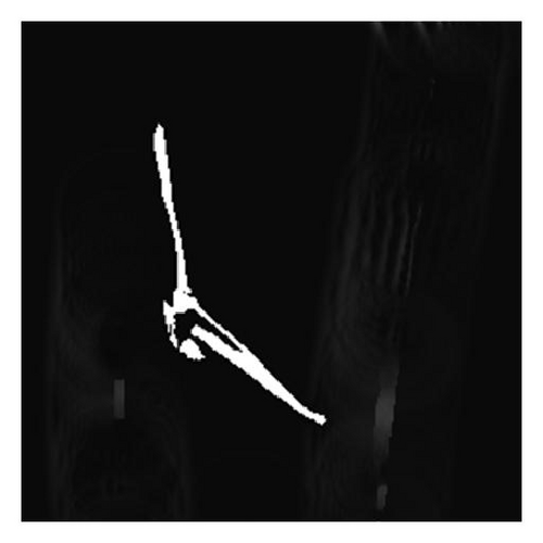
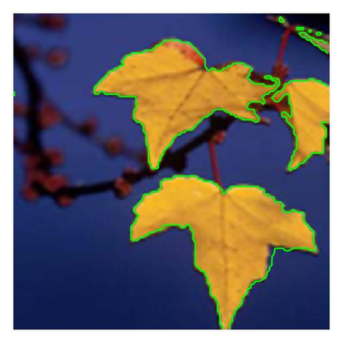
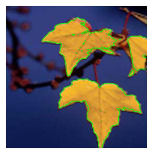
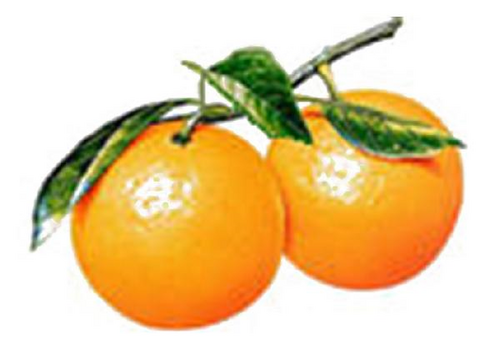
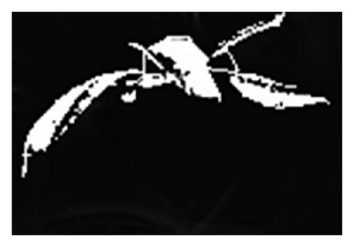
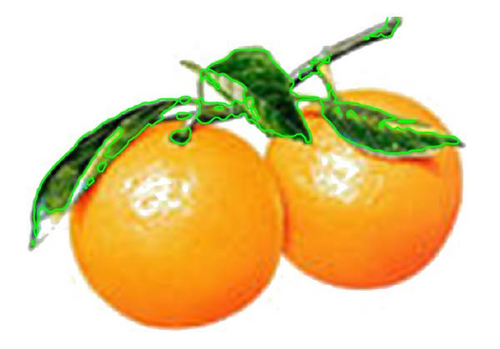
In the following, we compare our new model with the model [23] in Figures 3, 4, and 5. Figures 3(a), 4(a), and 5(a) are the original images. Our purpose is to segment the plane in Figure 3(a), the yellow leaves in Figure 4(a) and the green leaves of oranges in Figure 5(a). Figures 3(b), 4(b), 5(b), 3(c), 4(c), and 5(c) denote the final active contours and u obtained by using our new model, respectively. According to these results, we see that our model can detect the boundaries of the desired objects very accurately. And these results are hard to achieve by using the model in [23].







4. Conclusion
This paper describes a new variational model for segmenting desired objects in color images. This model is inspired by the GAC model, the region-scalable fitting model, the weighted bounded variation model and the active contour models based on the Mumford-Shah model. In order to segment objects of interest from color images, the energy functional in our model includes a discrimination function which determines whether an image pixel belongs to the desired objects or not. Compared with other active contour models, our new model cannot only avoid the usual drawback in the level set approach but also detect the desired objects accurately. Our numerical results confirm the effectiveness of our algorithm. Moreover, we establish the existence of the minimum to the new energy functional and analyze the property of it.
Acknowledgments
The authors wish to thank the referees for their valuable corrections and suggestions to the original manuscript. This work is supported by “the Fundamental Research Funds for the Central Universities” (Grant no. HIT. NSRIF. 2009049) and also supported by Natural Sciences Foundation of Heilongjiang Province (A200909).


