The covariance structure of spatial Gaussian predictors (aka Kriging predictors) is generally modeled by parameterized covariance functions; the associated hyperparameters in turn are estimated via the method of maximum likelihood. In this work, the asymptotic behavior of the maximum likelihood of spatial Gaussian predictor models as a function of its hyperparameters is investigated theoretically. Asymptotic sandwich bounds for the maximum likelihood function in terms of the condition number of the associated covariance matrix are established. As a consequence, the main result is obtained: optimally trained nondegenerate spatial Gaussian processes cannot feature arbitrary ill-conditioned correlation matrices. The implication of this theorem on Kriging hyperparameter optimization is exposed. A nonartificial example is presented, where maximum likelihood-based Kriging model training is necessarily bound to fail.

1. Introduction

Spatial Gaussian processing, also known as best linear unbiased prediction, refers to a statistical data interpolation method, which is nowadays applied in a wide range of scientific fields, including computer experiments in modern engineering context; see, for example, [1–5]. As a powerful tool for geostatistics, it has been pioneered by Krige in 1951 [6], and to pay tribute to his achievements, the method is also termed Kriging; see [7, 8] for geostatistical background.

In practical applications, the data′s covariance structure is modeled through covariance functions depending on the so-called hyperparameters. These, in turn, are estimated by optimizing the corresponding maximum likelihood function. It has been demonstrated by many authors that the accuracy of Kriging predictors relies both heavily on hyperparameter-based model training and, from the numerical point of view, on the condition number of the associated Kriging correlation matrix. In this regard, we relate to the following, nonexhaustive selection of papers: Warnes and Ripley [9] and Mardia and Watkins [10] present numerical examples of difficult-to-optimize covariance model functions. Ababou et al. [11] show that likelihood-optimized hyperparameters may correspond to ill-conditioned correlation matrices. Diamond and Armstrong [12] prove error estimates under perturbation of covariance models, demonstrating a strong dependence on the correlation matrix′ condition number. In the same setting, Posa [13] investigates numerically the behavior of this precise condition number for different covariance models and varying hyperparameters. An extensive experimental study of the condition number as a function of all parameters in the Kriging exercise is provided by Davis and Morris [14]. Schöttle and Werner [15] propose Kriging model training under suitable conditioning constraints. Related is the work of Ying [16] and Zhang and Zimmerman [17], who prove asymptotic results on limiting distributions of maximum likelihood estimators when the number of sample points approaches infinity. Radial basis function interpolant limits are investigated in [18]. Modern textbooks covering recent results are [19, 20].

In this paper, the connection between hyper-parameter optimization and the condition number of the correlation matrix is investigated from a theoretical point of view. The setting is as follows. All sample data is considered as fixed. An arbitrary feasible covariance model function is chosen for good, so that only the covariance models′ hyperparameters are allowed to vary in order to adjust the model likelihood. This is exactly the situation as it occurs in the context of computer experiments, where, based on a fixed set of sample data, predictor models have to be trained numerically. We prove that, under weak conditions, the limit values of the quantities in the model training exercise exist. Subsequently, by establishing asymptotic sandwich bounds on the model likelihood based on the condition number of the associated correlation matrix, it is shown that ill-conditioning eventually also decreases the model likelihood. This result implies a strategy for choosing good starting solutions for hyperparameter-based model training. We emphasize that all covariance models applied in the papers briefly reviewed above subordinate to the theoretical setting of this work.

The paper is organized as follows. In the next section, a short review of the basic theory behind Kriging is given. The main theorem is stated and proved in Section 3. In Section 4, an example of a Kriging data set is presented, which illustrates the limitations of classical model training.

2. Kriging in a Nutshell

Kriging is a statistical approach for estimating an unknown (scalar) function

(2.1)

based on a finite data set of sample locations x¹, …, xⁿ ∈ U ⊂ ℝ^d with corresponding responses y₁ : = y(x¹), …, y_n : = y(xⁿ) ∈ ℝ obtained from measurements or numerical computations. The collection of responses is denoted by

(2.2)

The function y : U → ℝ to be estimated is assumed to be the realization of an underlying random process given by a regression model and a random error function ϵ(x) with zero mean. More precisely

(2.3)

where the components of the row vector function f : ℝ^d → ℝ^p+1 are the basis functions of the regression model and β = (β₀, …, β_p) is the corresponding vector of regression coefficients. By assumption,

(2.4)

The component functions of f can be chosen arbitrarily, yet they should form a function basis suitable to the specific application. The most common choices for practical applications are

(1)
constant regression (ordinary Kriging): p = 0, f : ℝ^d → ℝ, x ↦ 1, f(x)β = β ∈ ℝ,
(2)
linear regression (universal Kriging): p = d, f : ℝ^d → ℝ^d+1, x ↦ (1, x₁, …, x_d), f(x)β = β₀ + β₁x₁ + ⋯+β_dx_d ∈ ℝ,

and higher-order polynomials.

Introducing the regression design matrix

(2.5)

the vector of errors at the sampled sites can be written as

(2.6)

Note that the first column of F equals 1 ∈ ℝⁿ for all polynomial regression models.

The Kriging predictor

estimates y at an untried site x as a linear combination of the sampled data

(2.7)

For each x ∈ ℝ^d, the unique vector of weights ω(x) = (ω₁(x), …, ω_n(x)) that leads to an unbiased prediction minimizing the mean squared error is given by the solution of the Kriging equation system

(2.8)

Here,

(2.9)

denote the covariance matrix and the covariance vector, respectively, and the entries of the vector μ = (μ₀, …, μ_p) are Lagrange multipliers. Solving (2.8) by Schur matrix complement inversion and substituting in (2.7) leads to the Kriging predictor formula

(2.10)

where β = (F^TR⁻¹F) ⁻¹F^TR⁻¹Y is the generalized least squares solution to the regression problem Fβ≃Y. For details, see, for example, [20, 21].

For setting up Kriging predictors, it is therefore mandatory to estimate the covariances based on the sampled data set. The two most popular approaches to tackle this problem are variogram fitting (the geostatistical literature, see [7]) and application of spatial correlation functions (computer experiments, see [4, 20]). The latter ones are usually of the form

(2.11)

Here θ = (θ₁, …, θ_d) ∈ ℝ^d is a vector of distance weights, which models the influence of the coordinate-wise spatial correlation on the prediction. The correlation matrix is defined by

(2.12)

In order to avoid ambiguity due to different parameterizations of the correlation models, we fix for the rest of the paper the following.

Convention 1 Large distance weight values correspond to weak spatial correlation, and small distance weight values correspond to strong spatial correlation. More precisely, we assume that feasible spatial correlation functions are always parameterized such that

(2.13)

at distinct locations p ≠ q.

All correlation models applied in all the papers briefly reviewed in the introduction can be parameterized accordingly. A collection of spatial correlation functions is given in several publications on Cokriging/Kriging, including [21, Table 2.1]. For example, the Gaussian correlation function parameterized with respect to the convention above is given by

(2.14)

The results and proofs presented below hold true without change for every admissible spatial correlation model, assuming that the sample errors are normally distributed and that the process variance is stationary; that is, σ is independent of the locations xⁱ, x^j. In this setting, hyper-parameter training for Kriging models consists of optimizing the corresponding maximum likelihood function

(2.15)

For θ fixed, optima for σ = σ(θ) and β = β(θ) can be derived analytically, see [20], so that hyper-parameter training for Kriging models is reduced to the following optimization problem:

(2.16)

where the dependency on θ is as follows:

(2.17)

(2.18)

(2.19)

Because the logarithm is monotonic, this is equivalent to minimizing the so-called condensed log-likelihood function

(2.20)

often encountered in the literature.

3. Asymptotic Behavior of the Maximum Likelihood Function—Why Kriging Model Training Is Tricky: Part I

The condition number of a regular matrix R ∈ ℝ^n×n with respect to a given matrix norm ∥·∥ is defined as cond(R): = ∥R∥·∥R⁻¹∥. For the matrix norm induced by the euclidean vector norm, one can show that

(3.1)

where λ_max, λ_min are the largest, the smallest eigenvalue of R, respectivley. In order to prevent the solution of the Kriging equation system (2.8) from being spoiled by numerical errors, it is important to prevent the covariance matrix from being severely ill-conditioned. However, the next theorem shows that eventually, when the condition number approaches infinity, so does the associated likelihood function. (Keep in mind that we have formulated likelihood estimation as a minimization problem; see (2.16).) Throughout this section, we will assume that the regression design matrix F from (2.5) features the vector 1 ∈ ℝⁿ as first column. This is the case of the highest practical relevance and, in fact, is of particular difficulty, since in this case the first column of F coincides with a limit eigenvector of the correlation matrix as will be seen in the following.

Theorem 3.1. Let x¹, …, xⁿ ∈ ℝ^d, Y : = (y(x¹), …, y(xⁿ)) ∈ ℝⁿ be a data set of sampled sites and responses. Let R(θ) be the associated spatial correlation matrix, and let Σ(θ) be the vector of errors with respect to the chosen regression model. Furthermore, let cond(R(θ)) be the condition number of R(θ). Suppose that the following conditions hold true:

(1)
the eigenvalues λ_i(θ) of R(θ) are mutually distinct for small 0 < ∥θ∥≤ɛ, θ ∈ ℝ^d,
(2)
the derivatives of the eigenvalues do not vanish in the limit: for all j = 2, …, n,
(3)
Σ(0) ∉ span {1}, Σ(0) ∉ 1^⊥.

Then,

(3.2)

and there exist constants c₁, c₂ ∈ ℝ such that

(3.3)

for θ ∈ ℝ^d, 0 < ∥θ∥≤ɛ. The constants c₁, c₂ are independent of θ.

Remark 3.2. (1) The conditions given in the above theorem cannot be proven to hold true in general, since they depend on the data set in question. However, they hold true for nondegenerate data set. In Appendix A, a relationship between condition 2 and the regularity of R′(0) is established, giving strong support that condition 2 is generally valid. Concerning the third condition, it will be shown in Lemma 3.4, that the limit Σ(0) exists, given conditions 1 and 2. Note that the set span {1} ∪ 1^⊥ is of Lebesgue measure zero in ℝⁿ. In all practical applications known to the author, these conditions were fulfilled.

(2) It holds that lim _{∥θ∥→∞}(R(θ)) _i,j = I ∈ ℝ^n×n. Hence, the likelihood function approaches a constant limit for ∥θ∥→∞ and lim _{∥θ∥→∞}cond(R(θ)) = 1. The corresponding predictor behavior is investigated in Section 4.

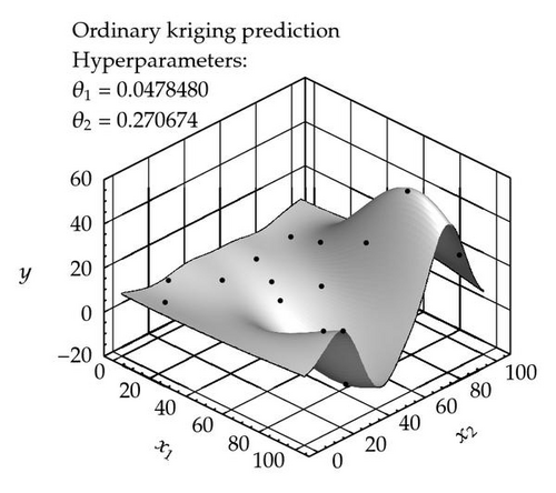
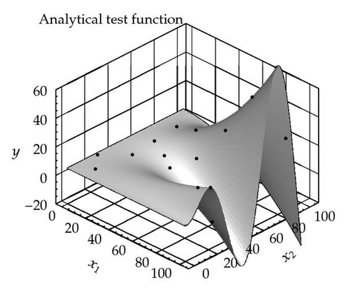
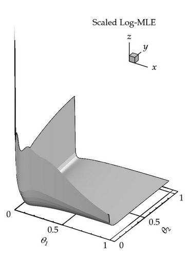
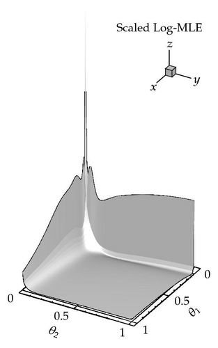
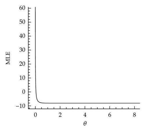
(3) Even though Theorem 3.1 shows that the model likelihood becomes arbitrarily bad for hyperparameters ∥θ∥→0, the optimum might lie very close to the blowup region of the condition number, leading to still quite ill-conditioned covariance matrices [11]. This fact as well as the general behavior of the likelihood function as predicted by Theorem 3.1 is illustrated in Figure 1.

(4) Figure 2(b), provides an additional illustration of Theorem 3.1.

(5) Theorem 3.1 offers a strategy for choosing starting solutions for the optimization problem (2.16): take each θ_k, k ∈ 1, …, d as small as possible such that the corresponding correlation matrix is still (numerically) positive definite.

(6) A related investigation of interpolant limits has been performed in [18] but for standard radial basis functions.

Details are in the caption following the image — **Figure 1 (a)**
Open in figure viewer PowerPoint

Ordinary Kriging estimation (a) of a two-dimensional analytical test function (b) based on 15 samples points. ((c) and (d)) Two views of the associated LogML, scaled by a factor of 1/100. This example shows that hyperparameter optima might lie very close to the blowup of the Log ML due to ill-conditioning, that is proved to occur by Theorem 3.1. Model function and sample locations are listed in Appendix B.

In order to support readability, we divide the proof of Theorem 3.1 into smaller units, organized as follows. As a starting point, we establish two auxiliary lemmata on the existence of limits of eigenvalue quotients and of errors vectors. Subsequently, the proof of the main theorem is conducted relying on the lemmata.

Lemma 3.3. In the setting of Theorem 3.1, let λ_i(θ), i = 1, …, n be the eigenvalues of R(θ), ordered by size. Then,

(3.4)

Proof. Because of (2.13), it holds that (R(0)) _i,j = 11^T ∈ ℝ^n×n for every admissible spatial correlation function. Since (11^T)1 = n1 ∈ ℝⁿ and (11^T)W = 0 for all W ∈ 1^⊥ ⊂ ℝⁿ, the limit eigenvalues of the correlation matrix ordered by size are given by λ₁(0) = n > 0 = λ₂(0) = ⋯ = λ_n(0).

Under the present conditions, the eigenvalues λ_i are differentiable with respect to θ. Hence, it is sufficient to proof the lemma for ℝ∋τ ↦ θ(τ) = τ1 ∈ ℝ^d and τ → 0. Now, condition 2 and L′Hospital′s rule imply the result.

Lemma 3.4. In the setting of Theorem 3.1, let Σ(θ) be defined by (2.18) and (2.19). Then,

(3.5)

exists.

Proof. We prove Lemma 3.4 by showing that lim _∥θ∥→0β(θ) exists.

Remember that β = (β₀, …, β_p) ^T ∈ ℝ^p+1, with p ∈ ℕ₀ depending on the chosen regression model. As in the above lemma, we can restrict the considerations to the direction τ ↦ θ(τ) = τ1.

Let λ_i(θ), i = 1, …, n be the eigenvalues of R(θ) ordered by size with corresponding eigenvector matrix Q(θ) = (X₁, …, X_n)(θ) such that Q(θ)R(θ)Q^T(θ) = Λ(θ) = diag (λ₁, …, λ_n). For brevity, define X_i(τ): = X_i(θ(τ)) = X_i(τ1) and so forth.

It holds that ; see Lemma 3.3. Hence, 〈1, X_j(τ)〉→0 for τ → 0 and j = 2, …, n. In the present setting, the derivatives of eigenvalues and (normalized) eigenvectors exist and can be extended to 0; see, for example, [22]. By another application of L′Hospital′s rule,

(3.6)

Introducing

(3.7)

we can restate (2.19) as

(3.8)

It is sufficient to show that lim _τ→0(LF^TQΛ⁻¹)(τ) exists.

Writing columnwise (F₀, F₁, …, F_p): = F, a direct computation shows

(3.9)

Note that

for the default choices of regression basis functions, such that 〈F₀, X₁(0)〉≠0 and 〈F₀, X_j(0)〉 = 0 for j = 2, …, n. The desired result follows from (3.6) and Lemma 3.3.

Remark 3.5. Actually, one cannot prove for (LF^TQΛ⁻¹) to be regular in general, since this matrix depends on the chosen sample locations. It might be possible to artificially choose samples such that, for example, F has not full rank. Yet if so, the whole Kriging exercise cannot be performed, since (2.19) is not well defined in this case. For constant regression, that is, F = 1, this is impossible. Note that F is independent of θ.

Now, let us prove Theorem 3.1 using notation as introduced above.

Proof. As shown in the proof of Lemma 3.3

(3.10)

Because the correlation matrix is symmetric and positive definite, a decomposition

(3.11)

with Q orthogonal and

, exists.

If necessary, renumber such that λ_max = λ₁ ≥ ⋯≥λ_n = λ_min. Let W(θ) = (W₁(θ), …, W_n(θ)): = Q(θ)Σ(θ). By Lemma 3.4, W(0): = Q(0) ^TΣ(0) exists. Condition 3 insures that W₁(0) ≠ 0.

Case 1. Suppose that W_i(0) ≠ 0 for all i = 1, …, n.

By continuity, W_i(θ) ≠ 0 for 0 ≤ ∥θ∥≤ɛ and ɛ > 0 small enough. Since {θ ∈ ℝ^d, 0 ≤ ∥θ∥≤ɛ} is a compact set,

(3.12)

exists. Then, for ∥θ∥∈[0, ϵ],

(3.13)

Case 2. Suppose that Case 1 does not hold true.

From Σ(0) ∉ span {1}, it follows that

(3.14)

for ∥θ∥ sufficiently small. Let J : = {i ∈ {1, …, n}∣W_i(0) ≠ 0}. Then, n_J : = |J | ≥ 2.

Define

(3.15)

For the index

defined by

, it holds that

By Lemma 3.3,

(3.16)

exists. Using

(3.17)

together with

(3.18)

the result can be established as in Case 1.

The estimate of the upper bound of ML is obtained in an analogous manner. Let

(3.19)

Then,

(3.20)

where we used Bernoulli′s inequality at (*), Lemma 3.3, and the fact that n/(n − 1) ≤ 2.

Remark 3.6. The extension of the main theorem to Cokriging prediction [7, 20] is a straight-forward exercise, since the limit eigenvectors of the Cokriging correlation matrix corresponding to nonzero eigenvalues can also be determined explicitly.

4. Why Kriging Model Training Is Tricky: Part II

The following simple observation illustrates Kriging predictor behavior for large-distance weights θ. Notation is to be understood as introduced in Section 3.

Observation 1. Suppose that sample locations {x¹, …, xⁿ} ⊂ ℝ^d and responses y_i = y(xⁱ) ∈ ℝ, i = 1, …, n are given. Let be the corresponding Kriging predictor according to (2.10). Then, for ℝ^d∋x ∉ {x¹, …, xⁿ} and distance weights ∥θ∥→∞, it holds that

(4.1)

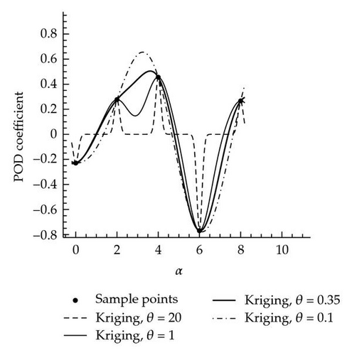
Put in simple words: if too large distance weights are chosen, then the resulting predictor function has the shape of the regression model, x ↦ f(x)β, with peaks at the sample sites, compare Figure 2, dashed curve.

Proof. According to (2.10) it holds that

(4.2)

where C = σ²R. By (2.13), it holds that R(θ) → I, for ∥θ∥→∞ for every admissible spatial correlation model of the form of (2.11). By Cauchy-Schwartz′ inequality,

(4.3)

where ∥c_θ(x)∥→0 and

. for ∥θ∥→∞.

Remark 4.1. The same predictor behavior arises at locations far away from the sampled sites, that is, for dist (x, {x¹, …, xⁿ}) → ∞. This has to be considered, when extrapolating beyond the sample data set.

Figure 2 shows an example data set for which the Kriging maximum likelihood function is constant over a large range of θ values. This example was not constructed artificially but occured in the author′s daily work of computing approximate fluid flow solutions based on proper orthogonal decomposition (POD) followed by coefficient interpolation as described in [23, 24].

The sample data set is given in Table 1. The Kriging estimator given by the dashed line shows a behavior as predicted by Observation 1. Note that from the model training point of view, all distance weights θ > 1 are equally likely, yet lead to quite different predictor functions. Since the ML features no local minimum, classical hyperparameter estimation is impossible.

Table 1. Sampled sites corresponding to the example displayed in Figure 2.

x = α:	0.0	2.0	4.0	6.0	8.0
y(x):	−0.229334	0.277018	0.455534	−0.769558	0.26634

Nomenclature

d ∈ ℕ:: Dimension of parameter space
n ∈ ℕ:: (Fixed) number of sample points
xⁱ ∈ ℝ^d:: ith sample location
y_i ∈ ℝ:: Sample value at sample location xⁱ
I ∈ ℝ^n×n:: Unit matrix
1 : = (1, …, 1) ^T ∈ ℝⁿ:: Vector with all entries equal to 1
:: ith standard basis vector
V^⊥ ⊂ ℝⁿ:: Subspace of all vectors orthogonal to V ∈ ℝⁿ
R ∈ ℝ^n×n:: Correlation matrix
C ∈ ℝ^n×n:: Covariance matrix
cond(R):: Condition number of R ∈ ℝ^n×n
〈·, ·〉:: Euclidean scalar product
e = exp (1):: Euler’s number
p + 1 ∈ ℕ:: Dimension of regression model
β ∈ ℝ^p+1:: Vector of regression coefficients
f : ℝ^d → ℝ^p+1:: Regression model
ϵ : ℝ^d → ℝ:: Random error function
E[·]:: Expectation value
:: Standard deviation
θ ∈ ℝ^d:: Distance weights vector, model hyperparameters.

Acknowledgments

This research was partly sponsored by the European Regional Development Fund and Economic Development Fund of the Federal German State of Lower Saxony Contract/Grant no. W3-80026826.

Appendices

A. On the Validity of Condition 2 in Theorem 3.1

The next lemma strongly indicates that the second condition in the main Theorem 3.1 is given in nondegenerate cases.

Lemma A.1. Let ℝ^d∋θ ↦ R(θ) ∈ ℝ^n×n be the correlation matrix function corresponding to a given set of Kriging data and a fixed spatial correlation model.

Let λ_i(θ), i = 1, …, n be the eigenvalues of R ordered by size with corresponding eigenvector matrix Q = (X₁, …, X_n), and define θ : ℝ → ℝ^d, τ ↦ θ(τ): = τ1. Suppose that the eigenvalues are mutually distinct for τ > 0 close to zero.

Denote the directional derivative in the direction 1 with respect to τ by a prime ′, that is, (d/dτ)R(τ1) = R′(τ) and so forth. Then, it holds that

(A.1)

If R′(0) is regular, then

(A.2)

for all i = 1, …, n, with at most one possible exception.

Proof. For every admissible spatial spatial correlation function r(θ, ·, ·) of the form (2.11) and x ≠ z ∈ ℝ^d, it holds that

(A.3)

Thus, (R(0)) _i,j = 11^T ∈ ℝ^n×n.

It holds that (11^T)1 = n1 ∈ ℝⁿ and (11^T)W = 0 for all W ∈ 1^⊥ ⊂ ℝⁿ; therefore, the limits of the eigenvalues of the correlation matrix ordered by size are given by λ₁(0) = n > λ₂(0) = ⋯ = λ_n(0) = 0. The assumption, that no multiple eigenvalues occur, ensures that the eigenvalues λ_i and corresponding (normalized, oriented) eigenvectors X_i are differentiable with respect to τ. Let Q(τ) = (X₁(τ), …, X_n(τ)) ∈ ℝ^n×n be the (orthogonal) matrix of eigenvectors, such that

(A.4)

Then,

(A.5)

where Q(0) is the continuous extension of Q(τ); see, for example, [22].

Hence,

(A.6)

Let us assume, that there exist two indices j₀, k₀, j₀ ≠ k₀ such that .

Let . Then,

(A.7)

contradicting the regularity of R′(0), if W ≠ 0.

If W = 0, replace W by and repeat the above argument.

For most correlation models, the derivative R′(0) can be computed explicitly.

B. Test Setting Corresponding to Figure 1

In order to produce Figure 1, the following test function has been applied:

(B.1)

The Kriging predictor function displayed in this figure has been constructed based on the fifteen (randomly chosen) sample points shown in Table 2.

Location	x₁	x₂	y(x₁, x₂)
1	84.0188	39.4383	−15.0146
2	78.3099	79.844	53.5481
3	91.1647	19.7551	20.0921
4	33.5223	76.823	13.506
5	27.7775	55.397	2.10686
6	47.7397	62.8871	5.07917
7	36.4784	62.8871	−1.23344
8	95.223	51.3401	26.5839
9	63.5712	71.7297	27.5219
10	14.1603	60.6969	4.74213
11	1.63006	24.2887	5.00422
12	13.7232	80.4177	6.48784
13	15.6679	40.0944	4.24907
14	12.979	10.8809	5.16235
15	99.8925	21.8257	22.8288

References

1 Han Z. H., Gortz S., and Zimmermann R., On improving efficiency and accuracy of variable-fidelity surrogate modeling in aero-data for loads context, Proceeings of European Air and Space Conference (CEAS ′09), October 2009, Manchester, UK.
Google Scholar
2 Kennedy M. C. and O′Hagan A., Predicting the output from a complex computer code when fast approximations are available, Biometrika. (2000) 87, no. 1, 1–13, 2-s2.0-0007312235.
10.1093/biomet/87.1.1
Web of Science® Google Scholar
3 Laurenceau J. and Sagaut P., Building efficient response surfaces of aerodynamic functions with kriging and cokriging, AIAA Journal. (2008) 46, no. 2, 498–507, 2-s2.0-43649093003, https://doi.org/10.2514/1.32308.
10.2514/1.32308
Web of Science® Google Scholar
4 Sacks J., Welch J., Mitchell T. J., and Wynn H., Design and analysis of computer experiments, Statistical Science. (1989) 4, no. 4, 409–423.
10.1214/ss/1177012413
Google Scholar
5 Zimmermann R. and Han Z. H., Simplified cross-correlation estimation for multi-fidelity surrogate cokriging models, Advances and Applications in Mathematical Sciences. (2010) 7, no. 2, 181–202.
Google Scholar
6 Krige D., A statistical approach to some basic mine valuation problems on the Witwa-tersrand, Journal of the Chemical, Metallurgical and Mining Engineering Society of South Africa. (1951) 52, no. 6, 119–139.
Google Scholar
7 Journel A. G. and Huijbregts C. J., Mining Geostatistics, 1991, 5th edition, The Blackburn Press, Caldwell, NJ, USA.
Google Scholar
8 Matheron G., Principles of geostatistics, Economic Geology. (1963) 58, 1246–1266.
10.2113/gsecongeo.58.8.1246
CAS Google Scholar
9 Warnes J. J. and Ripley B. D., Problems with likelihood estimation of covariance functions of spatial Gaussian processes, Biometrika. (1987) 74, no. 3, 640–642, https://doi.org/10.1093/biomet/74.3.640.
10.1093/biomet/74.3.640
Web of Science® Google Scholar
10 Mardia K. V. and Watkins A. J., On multimodality of the likelihood in the spatial linear model, Biometrika. (1989) 76, no. 2, 289–295, https://doi.org/10.1093/biomet/76.2.289.
10.1093/biomet/76.2.289
Web of Science® Google Scholar
11 Ababou R., Bagtzoglou A. C., and Wood E. F., On the condition number of covariance matrices in kriging, estimation, and simulation of random fields, Mathematical Geology. (1994) 26, no. 1, 99–133, 2-s2.0-0028322792, https://doi.org/10.1007/BF02065878.
10.1007/BF02065878
Web of Science® Google Scholar
12 Diamond P. and Armstrong M., Robustness of variograms and conditioning of kriging matrices, Journal of the International Association for Mathematical Geology. (1984) 16, no. 8, 809–822, 2-s2.0-0000755164, https://doi.org/10.1007/BF01036706.
10.1007/BF01036706
Web of Science® Google Scholar
13 Posa D., Conditioning of the stationary kriging matrices for some well-known covariance models, Mathematical Geology. (1989) 21, no. 7, 755–765, 2-s2.0-0000197738, https://doi.org/10.1007/BF00893320.
10.1007/BF00893320
Google Scholar
14 Davis G. J. and Morris M. D., Six factors which affect the condition number of matrices associated with kriging, Mathematical Geology. (1997) 29, no. 5, 669–683, 2-s2.0-0031473268.
10.1007/BF02769650
Google Scholar
15 Schöttle K. and Werner R., Improving the most general methodology to create a valid correlation matrix, Management Information Systems. (2004) 9, 701–710.
Google Scholar
16 Ying Z., Asymptotic properties of a maximum likelihood estimator with data from a Gaussian process, Journal of Multivariate Analysis. (1991) 36, no. 2, 280–296, 2-s2.0-0004770346.
10.1016/0047-259X(91)90062-7
Web of Science® Google Scholar
17 Zhang H. and Zimmerman D. L., Towards reconciling two asymptotic frameworks in spatial statistics, Biometrika. (2005) 92, no. 4, 921–936, 2-s2.0-27944497893, https://doi.org/10.1093/biomet/92.4.921.
10.1093/biomet/92.4.921
Web of Science® Google Scholar
18 Buhmann M. D., Dinew S., and Larsson E., A note on radial basis function interpolant limits, IMA Journal of Numerical Analysis. (2010) 30, no. 2, 543–554, 2-s2.0-77950234353, https://doi.org/10.1093/imanum/drn051.
10.1093/imanum/drn051
Web of Science® Google Scholar
19 Rasmussen C. E. and Williams C. K. I., Gaussian Processes for Machine Learning, 2006, MIT Press, Cambridge, Mass, USA.
Google Scholar
20 Santner T. J., Williams B. J., and Notz W. I., The Design and Analysis of Computer Experiments, 2003, Springer, New York, NY, USA.
10.1007/978-1-4757-3799-8
Google Scholar
21 Lophaven S., Nielsen H. B., and Søndergaard J., DACE—a MATLAB kriging tool-box, version 2.0, 2002, no. IMM-TR-2002-12, Technical University of Denmark.
Google Scholar
22 van der Aa N. P., Ter Morsche H. G., and Mattheij R. R. M., Computation of eigenvalue and eigenvector derivatives for a general complex-valued eigensystem, Electronic Journal of Linear Algebra. (2007) 16, 300–314, 2-s2.0-34948836292.
10.13001/1081-3810.1203
Web of Science® Google Scholar
23 Zimmermann R. and Gortz S., Non-linear reduced order models for steady aerodynamics, Procedia Computer Sciences. (2010) 1, no. 1, 165–174.
10.1016/j.procs.2010.04.019
Google Scholar
24 Bui-Thanh T., Damadoran M., and Willcox K., Proper orthogonal decomposition extensions for parametric applications in transonic aerodynamics, Proceedings of the 21th AIAA Applied Aerodynamics Conference, 2003, Orlando Fla, USA, AIAA paper 2003-4213.
Google Scholar

Citing Literature

All articles

Asymptotic Behavior of the Likelihood Function of Covariance Matrices of Spatial Gaussian Processes

Abstract

1. Introduction

2. Kriging in a Nutshell

3. Asymptotic Behavior of the Maximum Likelihood Function—Why Kriging Model Training Is Tricky: Part I

4. Why Kriging Model Training Is Tricky: Part II

Nomenclature

Acknowledgments

Appendices

A. On the Validity of Condition 2 in Theorem 3.1

B. Test Setting Corresponding to Figure 1

References

Citing Literature

Figures

References

Information

About Wiley Online Library

Help & Support

Opportunities

Connect with Wiley