Volume 2010, Issue 1 375615
Research Article
Open Access

Forward Sensitivity Approach to Dynamic Data Assimilation

S. Lakshmivarahan

Corresponding Author

S. Lakshmivarahan

School of Computer Sciences University of Oklahoma Norman, OK 73072, USA , ou.edu

Search for more papers by this author
J. M. Lewis

J. M. Lewis

Forecast R&D National Severe Storms Laboratory Norman, OK 73072, USA , noaa.gov

Division of Atmospheric Sciences Desert Research Institute Reno, NV 89512, USA , dri.edu

Search for more papers by this author
First published: 05 May 2010
Citations: 18
Academic Editor: Zhaoxia Pu

Abstract

The least squares fit of observations with known error covariance to a strong-constraint dynamical model has been developed through use of the time evolution of sensitivity functions—the derivatives of model output with respect to the elements of control (initial conditions, boundary conditions, and physical/empirical parameters). Model error is assumed to stem from incorrect specification of the control elements. The optimal corrections to control are found through solution to an inverse problem. Duality between this method and the standard 4D-Var assimilation using adjoint equations has been proved. The paper ends with an illustrative example based on a simplified version of turbulent heat transfer at the sea/air interface.

1. Introduction

Sensitivity function analysis has proved valuable as a mean to both build models and to interpret their output in chemical kinetics (Rabitz et al. [1], Seefeld and Stockwell [2]) and air quality modeling (Russell et al. [3]). Yet, the ubiquitous systematic errors that haunt dynamical prediction cannot be fully understood with sensitivity functions alone. We now include an optimization component that leads to an improved fit of model to observations. The methodology is termed forward sensitivity method (FSM)—a method based on least squares fit of model to data, but where algorithmic structure and correction procedure are linked to the sensitivity functions. In essence, corrections to control (the initial conditions, the boundary conditions, and the physical and empirical parameters) are found through solution to an inverse problem.

In this paper we derive the governing equations for corrections to control and show their equivalence to equations governing the so-called 4D-Var assimilation method (four-dimensional variational method)—least squares fit of model to observations under constraint (LeDimet and Talagrand [4]). Beyond this equivalence, we demonstrate the value of the FSM as a diagnostic tool that can be used to understand the relationship between sensitivity and correction to control.

We begin our investigation by laying down the dynamical framework for the FSM: general form of the governing dynamical model, the type and representation of model error that can identified through the FSM, and the evolution of the sensitivity functions that are central to execution of the FSM. The dual relationship between 4D-Var/adjoint equations is proved. The step-by-step process of assimilating data by FSM is outlined, and we demonstrate its usefulness by application to a simplified air-sea interaction model.

2. Foundation Dynamics for the FSM

We have included a list of mathematical symbols used in this paper. These symbols and associated nomenclature are found in Table 1.

Table 1. Symbolism and nomenclature.
Symbol Nomenclature
n Dimension of state vector
m Dimension of observation vector
p Dimension of parameter vector
q = n + p Dimension of control vector
N Number of observation vectors
t Time
True model state vector
x(t) = (x1, x2, …xn) TRn Model state vector
f : Rn × Rp Vector field of the model
x(0) ∈ Rn Initial condition for model state vector
αRp Parameter vector
c = (x(0), α) ∈ Rn × Rp Control vector
z(t) ∈ Rm Observation vector
h(x(t)) : RnRm Forward operator relating model state and observations
h(x(t)) ∈ Rm Model counterpart of the observation
v(t) ∈ Rm Observation error vector
R(t) ∈ Rm×n Covariance of observation error vector v(t)
eF Forecast error
b(t) Systematic component of forecast error
Dx(f) = [fi/xj] ∈ Rn×n Model Jacobian w. R. T. x
Dα(f) = [fi/αj] ∈ Rn×p Model Jacobian w. R. T. A
Dα(x) = [xi/αj] ∈ Rn×p Sensitivity matrix w. R. T. Parameters
Dx(0)(x) = [xi/xj(0)] ∈ Rn×n Sensitivity matrix w. R. T. Initial condition
Dx(h) ∈ Rm×n Jacobian of the forward operator w. R. T. X
H1(t) = Dx(h)Dx(0)(x) ∈ Rm×n Sensitivity matrix accounting for h(x(t))
H2(t) = Dx(h)Dα(x) ∈ Rm×p Sensitivity matrix accounting for h(x(t))
a, b Inner product
J(c), J1(c) Objective or cost functions
δJ, δJ1, δx(t), δα First variations
J, ∇J1 Gradients of cost functions
M(t, s) Model state transition matrix (Appendix A)
L(t, s) Matrix that determines particular solution (Appendix A)

2.1. Prediction Equations

Let x(t) ∈ Rn denote the state and let αRpdenote the parameters of a deterministic dynamical system, where x(t) = (x1(t), x2(t), …, xn(t)) T and α = (α1, α2, …, αp) T are column vectors, n and p are positive integers, t ≥ 0 denotes the time, and superscript T denotes the transpose of the vector or matrix. Let f : Rn × Rp × RRn be a mapping, where f(x, α, t) = (f1, f2, …, fn) T with fi = fi(x, α, t) for 1 ≤ in. The vector spaces Rn and Rp are called the model space and parameter space, respectively.

Consider a dynamical system described by a system of ordinary nonlinear differential equations of the form
(1a)
or in component form
(1b)
where dx/dt denotes the time derivative of the state x(t), with x(0) ∈ Rn the given initial condition. The control vector for the model is given by c = (x(0), α) ∈ Rn × Rp, the combination of initial condition and parameters referred to as the control space. It is tacitly assumed that the map of f in (1a) and (1b) is such that the solution x(t) = x(t, x(0), α) = x(t, c) exists and is unique. It is further assumed that x(t) has a smooth dependence on the control vector c such that the first k (≥1) partial derivatives of x(t) with respect to the components of c also exist. The solution x(t) of (1a) and (1b) is known as the deterministic forecast of the state of the system at time t > 0. If the map f(·) in (1a) and (1b) depends explicitly on t, then this system is called a time varying or nonautonomous system; if f(·) does not depend on t, then the system is known as a time invariant or autonomous system.

Let z(t) ∈ Rm be the observation vector obtained from the field measurements at time t ≥ 0. Let h : RnRm be the mapping from the model space Rn to the observation space Rm.

If denotes the (unknown) true state, then we assume that z(t) is given by
(2)
where v(t) ∈ Rm is the additive (unobservable and unavoidable) noise. The mapping h(·) is known as the forward operator or the observation operator. It is further assumed that v(t) is a white Gaussian noise with mean zero possessing a known covariance matrix R(t) ∈ Rm×m. That is, v(t) ~ N(0, R(t)).

2.2. A Classification of Forecast Errors

The forecast error eF(t) ∈ Rm is defined as follows:
(3)
the sum of a deterministic part
(4)
and the random part v(t) induced by the observation noise. Our immediate goal is to analyze and isolate sources and types of forecast errors.
First, if the model map f(·) and the forward operator h(·) are without error, that is, exact, and if the control vector c is also error free, then the deterministic forecast x(t) must be correct in the sense that , the true state. Then from (3), the forecast error is purely random or white Gaussian noise. That is,
(5)
Second, if f(·) and h(·) are known perfectly but c has an error, then the forecast x(t) will have a deterministic error induced by the incorrect control vector. In such a case, we can, in principle, decompose the forecast error as a sum
(6)
where the deterministic part, is purely a function of the control vector error.
Third, if f(·), h(·), and c are in error, then the forecast error can be represented as
(7)
where the deterministic part b(c, f, h, t) may have a complex (additive and/or multiplicative) dependence on errors in c, f(·), and h(·).

The following assumption is key to our analysis that follows. The model of choice is faithful to the phenomenon under study. The system is predicted with fidelity—the forecasted state is creditable and useful in understanding the dynamical processes that underpin the phenomenon. Certainly, the forecast will generally exhibit some error, but the primary physical processes are included; that is, the vector field fincludes the pertinent physical processes. In this situation the forecast error stems from erroneously specified elements of control. Thus, in our study the forecast error assumes the form shown in (6). Dee’s work [5] contains a very good discussion of the estimation of the bias b in (7) arising from errors in the model and/or observations.

2.3. Dynamics of First-Order Sensitivity Function Evolution

Since our approach is centered on sensitivity functions, we develop the dynamics of evolution of the forward sensitivities in this section.

Differentiating both sides of (1b) with respect to αj, interchanging the order of differentiation on the left-hand side, we obtain
(8)
for 1 ≤ in and 1 ≤ jp with xi(0)/αj = 0 as the initial condition.
These np equations can be succinctly written in matrix form as
(9)
with Dα(x(0)) = 0 as initial condition. This system of linear time-varying ordinary nonhomogeneous differential equations describe the evolution of the elements of Dα(x) = [xi/αj] ∈ Rn×p, where the Jacobian matrices Dx(f) ∈ Rn×n and Dα(f) ∈ Rn×p are given by
(10)
(11)
Similarly, by differentiating both sides of (1b) with respect to xj(0), we obtain
(12)
for 1 ≤ i, jn, with xi(0)/xj(0) = δij, where δij is the standard Kronecker delta. These n2 equations can be succinctly represented as
(13)
with Dx(0)(x(0)) = I, the identity matrix. This system of linear, time-varying homogeneous equations governs the evolution of the elements of the matrix Dx(0)(x) = [xi/xj(0)] ∈ Rn×p. Notice that (9) and (13) are independent of the observations and have the same system matrix Dx(f) on the right-hand sides; thus, the homogeneous solutions to (9) and (13) have the same structure.

The evolution of the sensitivities (solution to (9) and (13)) is dependent on the solution to the governing dynamical equations ((1a) and (1b)). Generally, these equations are solved numerically using the standard fourth-order Runge-Kutta method. Rabitz et al. work [1] contains more details relating to solutions of (9) and (13). In special cases such as in air quality modeling, the sensitivity equations (9) and (13) exhibit extreme stiffness. Special methods are needed to handle the inherent stiffness of these equations. Seefeld and Stockwell work [2] includes a discussion of these issues. Gear’s work [6] is a good reference for a general discussion of stiff equations.

3. Duality between the FSM and 4D-Var Based on Adjoint Method

Let z(t1), z(t2), …, z(tN) be a sequence of N observation vectors at times t0 = 0 < t1 < t2 ⋯ <tN. The goal is to use these observations to improve the estimate of the control vector c. This estimation problem is recast as a constrained minimization of an objective function J : Rn × RpR given by
(14)
where the model state x(t) evolves according to (1a), (1b), and R(ti) ∈ Rm×m is the known covariance of the observational errors v(ti) at time ti, 1 ≤ iN.
Fundamental to minimizing (14) is the computation of the gradient of J(c), denoted by ∇cJ(c). In the following we describe two ways of characterizing
(15)
where ∇x(0)JRn and ∇αJRp.

3.1. The Adjoint Method

This method is based on the basic principle that if δJ is the first variation of J(c) induced by the perturbation δc in c, then
(16)
where 〈a, b〉 denotes the standard inner product of two vectors a and b of the same dimension. Once the first variation δJ is determined, the gradient can be found. In the following we exploit two basic properties of inner product:
(i) linearity
(17)
(ii) adjoint property
(18)
where GT is the transpose or the adjoint of the matrix G.
From first principles (Chapter 24 in Lewis et al. [7]), it can be verified that the first variation δJ of J in (14) is given by
(19)
where the forecast error given by
(20)
is the Jacobian of forward operator h(x) with respect to x.
By invoking the adjoint property in (17), (19) becomes
(21)
where
(22)
The first variation δx(tk) in x(t) at t = tk resulting from the perturbation δc in c is given by (A.4) in Appendix A. Using (A.4) and the linearity of the inner product it follows that
(23)
where we will refer to the first term on the right-hand side of (23) as “Term I” and the second as “Term II.” Using the adjoint and linearity property in (17), we get
(24)
from which we obtain
(25)
Similarly, rewriting Term II as
(26)
we get
(27)
Hence, we obtain the components of ∇cJ which are used in conjunction with the minimization algorithm to find the optimal c* that minimizes J(c) in (14).
We conclude this discussion with an efficient recursive method for evaluating the expressions in (25) and (27). Define
(28)
and for k = N − 1, N − 2, …, 2,1, 0,
(29)
It can be verified that ∇x(0)J = MT(t1, 0)λ1 in (25).

Details on the recursive computation of (27) are given in Appendix C.

3.2. Sensitivity-Based Approach

Let us first consider the special case when N = 1. Then (14) becomes
(30)
where we recall that cRn × Rp and x = x(t, c) is the solution of the model equations (1a) and (1b) at time t.
Setting q = (n + p) and A = R−1(t), the expression J1(c) in (30) becomes identical to Q(c) in (B.16) (Appendix B). Hence, by using (B.20) it follows that
(31)
where η(t) is given by (22) and
(32)
Now comparing (32) with (25)–(27), we obtain the duality relation:
(33)
The sensitivity matrices on the left-hand side of (33) are obtained by solving the forward sensitivity equations, whereas the matrix products M(t, 0) and L(t, 0) are obtained by integrating along the path as given by (A.3) and (A.5) (Appendix A).

The primary advantage of the sensitivity-based approach is that it provides a natural interpretation of the expression for the gradient in (31). Recall from (22) that η(t) ∈ Rn is the weighted version of the forecast error R−1(t)eF(t) ∈ Rm mapped onto the model space by the linear operator . Also the ith column of is the sensitivity of the ith component xi(t) of the state vector x(t) ∈ Rn with respect to the control vector cRq given by (xi/c1, xi/c2, …, xi/cq). Thus, it follows from (31) that ∇cJ1 is a linear combination of the columns of which are the sensitivity vectors, where the coefficients of the linear terms are the components of η(t). Thus, columns of with large norms that are associated with large forecast errors will be dominant in determination of the components of ∇J1(c). In other words, we gain some insight into the interplay between corrections to control and forecast errors—something that can be seen through a careful examination of the sensitivity vector at various times from initial state to forecast horizon. (The illustrative example in Section 5 further explores this diagnostic function.) Expression (31) also enables us to isolate the effect of different components xi of x(t) on the performance index J1(c).

For the general case of observations at multiple times, (31) assumes the following form:
(34)
This gradient is the sum of linear combinations of the columns of at various time instances. With so many directions (the directions associated with the columns of contributing to the components of ∇cJ, the connection between sensitivity, and forecast error is obscured.

4. Data Assimilation Using Sensitivity

We seek to find the solution to the following problem using the FSM. Given f(·) and h(·), the control vector c, the observation z(t), and the error covariance of observations R(t), find a correction δc to the control vector such that the new model forecast starting from (c + δc) will render the forecast error eF(t) purely random; that is, the systematic forecast error is removed and accordingly E(eF(t)) = 0.

We start by quantifying the change Δx in the solution x(t) = x(t, c) resulting from a change δc in c. Invoking the standard Taylor series expansion, we obtain
(35)
where δkx is the kth variation of x(t), the fraction of the total change that can be accounted by the kth partial derivatives of x(t) with respect to c and the perturbation δc. Since practical considerations dictate that the total number of correction terms on the right-hand side of (35) be finite, we often settle for an approximation of only k terms (k generally ≤ 2). This is a tradeoff between improved accuracy resulting from a large value of k and the complexity of the resulting inverse problem. Although we have developed the methodology for second-order analysis (k = 2, where Δx is approximated by the sum δx + δ2x) (Lakshmivarahan and Lewis [8]), our development will follow the first-order analysis (k = 1, where Δx is given by the first variation δx). Second-order analysis is justified when δ2x is a significant fraction of δx—this occurs when f(x) and/or h(x) exhibit strong nonlinearity. It is further shown in Section 5 that iterative application of the first-order method often leads to improved results.

4.1. First-Order Analysis

From first principles and (35) we obtain
(36)
where Dx(0)(x) ∈ Rn×n is the Jacobian of x(t) with respect to x(0), and Dα(x) ∈ Rn×p is the Jacobian of x(t) with respect to α.The matrices Dx(0)(x) and Dα(x), found as solutions of (13) and (9), respectively, are known as the first-order sensitivity of the solution x(t) with respect to x(0) and α, respectively, and the elements of these matrices are called sensitivity functions.

4.1.1. Observations at One Time Only

We first consider the case where observation z(t) ∈ Rm is available at one time t. The first variation δx in x(t) induces a variation Δh in the forward operator h(x(t)). Again, by approximating Δh by the first variation, we get
(37)
where Dx(h) ∈ Rm×n is the Jacobian of h(·) with respect to x and is given by
(38)
substituting (36) into (37), we obtain
(39)
where H1(t) = Dx(h)Dx(0)(x) ∈ Rm×n and H2(t) = Dx(h)Dα(x) ∈ Rm×p. Setting H(t) = [H1(t), H2(t)] ∈ Rm×(n+p) and ς = (ς1, ς2) ∈ Rn+p, where ς1 = δx(0) and ς2 = δα, (39) becomes
(40)
Given the operating point c, our goal is to find the perturbation δc such that the observation is equal to the model counterpart, that is,
(41)
or
(42)
From (43), it follows that the required perturbation ςRn+p is obtained by solving the linear inverse problem
(43)
where H(t) ∈ Rm×(n+p) and eF(t) ∈ Rm.

4.1.2. Observations at Multiple Times

The above analysis can be readily extended to the case where observations are available at N times. We denote these sets of observation vectors by z(t1), z(t2), …, z(tN), where 0 < t1 < t2 < ⋯<tN. The forecast error eF(ti) is given by
(44)
Define
(45)
Then at time ti we have
(46)
where
(47)
Now define a matrix HRNm×(n+p) and a vector eFRNm as
(48)
Then, the N relations in (46) can be succinctly denoted by
(49)
A number of special cases arise depending on (a) the value of Nm relative to (n + p), namely, over (under) determined cases when Nm > (<)(n + p) and (b) the rank of the matrix H(t), namely, H(t) is of full rank or rank deficient. In all these cases, the linear inverse problem (43) is recast as a minimization problem using the standard least squares framework (Lawson and Hanson [9]). The resulting minimization problem can then be solved using one of many standard methods, for example, the conjugate gradient method (Lewis et al. [7]; Nash and Sofer [10]).
As an illustration, consider the case when Nm > (n + p) and that the rank of H is (n + p), that is, full rank. The solution ς is then obtained by minimizing the weighted least squares criterion
(50)
where
(51)
is an Nm × Nm diagonal matrix with R(ti) as its ith diagonal block.
Although it is computationally efficient to minimize (50) by using a method like conjugate gradient, there is an advantage to analyze the properties of the optimal solution via the classical approach, that is, by setting the gradient of JN(ς) to zero. It can be verified that the minimizing JN is found by solving the symmetric linear system
(52)
or succinctly as
(53)
where H, eF, and R are defined in (48) and (51), and subscript “LS” refers to the least squares solution.

From the discussion relating to the classification of forecast errors, recall that the forecast error inherits its randomness from the (unobservable) observation noise. The vector eF on the right hand side of (53) is random and hence the solution ς of (53) is also random.

Since we are interested in forecast errors in response to incorrect control, we have
(54)
Now define
(55)
Hence, the vector eF in (48) can be expressed as
(56)
with E(eF) = b since E(v) = 0. Substituting (56) into (53) and taking the expectation give
(57)
Thus, the expected value of the correction to control is indeed a linear function of the forecast error b itself. It can be verified (Lewis et al. [7]) that the covariance of the least squares estimate [(53)] is given by
(58)
where ∇2JN(ς) is the Hessian of JN(ς) in (50).

5. A Practical Example: Air/Sea Interaction

We choose a simple but nontrivial differential equation to demonstrate the applicability of the forward-sensitivity method to identification of error in a dynamical model. We break this discussion into three parts as follows: (1) the model, (2) discussion of the diagnostic value of FSM, and (3) numerical experiments with data assimilation using FSM.

5.1. The Model

Consider the case where cold continental air moves out over an ocean of constant surface temperature. We follow a column of air in a Lagrangian frame; that is, the column of air moves with the prevailing low-level wind speed. Turbulent transfer of heat from the ocean to air warms the column. The governing equation is taken to be
(59)
where
  • θ: temperature of the air column ( C),

  • θs: temperature of the sea surface ( C),

  • CT: turbulent heat exchange coefficient (nondimensional),

  • V: speed of air column (ms−1),

  • H: height of the column (mixed layer)(m),

  • τ: time (h).Equation (59) is nondimensionalized by the following scaling:

(60)
The governing equation then takes the form
(61)
Assuming H ~ 150 m, V ~ 10 ms−1, CT ~ 10−3, then
(62)
Thus, we take our governing equation to be
(63)
where k = 0.25. The solution to (63) is
(64)
with c = (x(0), α) ∈ R × R2, and α = (xs, k) TR2, that is, n = 1 and p = 2. The solution depends linearly on x(0) and xs but nonlinearly on k.

There are three elements of control: initial condition, x(0), boundary condition, xs, and parameter, k.

5.2. Diagnostic Aspects of FSM
The Jacobians of f with respect to x and α are given by
(65)
and the Jacobians of the solution x(t) with respect to α and x(0) are given by
(66)
From (9) and (13) the evolution of the forward sensitivities is given by
(67)
(68)
(69)
where
(70)
Either by solving (67)–(70) or by computing directly from (64), it can be verified that the required sensitivities evolve according to
(71)
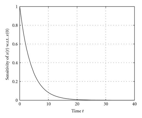
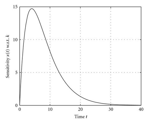
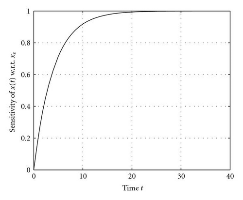
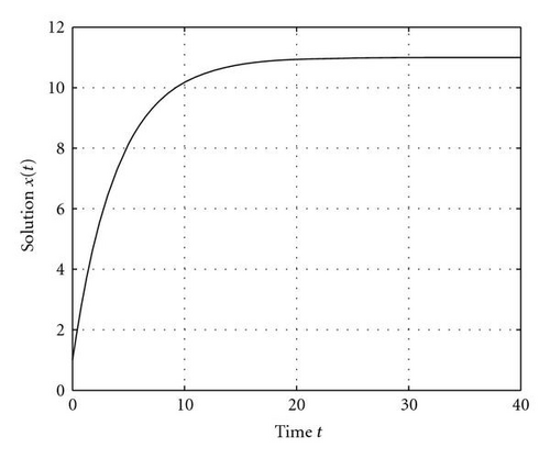
The plots of the solution and the three sensitivities are given in Figure 1.
Details are in the caption following the image
Figure 1 (a) Solution x(t)
Evolution of the solution of x(t) and its sensitivities to c = (x(0), xs, k) = (1.0, 11.0, 0.25).
Details are in the caption following the image
Figure 1 (b) Sensitivity of x(t) w.r.t. x(0)
Evolution of the solution of x(t) and its sensitivities to c = (x(0), xs, k) = (1.0, 11.0, 0.25).
Details are in the caption following the image
Figure 1 (c) Sensitivity of x(t) w.r.t. k
Evolution of the solution of x(t) and its sensitivities to c = (x(0), xs, k) = (1.0, 11.0, 0.25).
Details are in the caption following the image
Figure 1 (d) Sensitivity of x(t) w. r. t xs
Evolution of the solution of x(t) and its sensitivities to c = (x(0), xs, k) = (1.0, 11.0, 0.25).
Let z(t) be the direct observation of the state x(t), namely,
(72)
In this case, h(t) is the forecast variable and therefore Dx(h) = 1. Then
(73)
is the forecast error.
Following the developments in Section 4 for the case of a single observation described by (39)–(46), we obtain the analog of (46) as
(74)
where H = H(t) = [x(t)/x(0), x(t)/xs, x(t)/k] is the forward sensitivity vector and ς = [δx(0), δxs, δk] T. Clearly, (74) corresponds to an under-determined linear least squares problem, whose optimal solution is given by [7, chapter 5]
(75)
where HT/∥H∥ is the unit forward sensitivity vector at time t and eF(t)/∥H∥ is a scalar that is the forecast error normalized by the norm of the forward sensitivity vector H. In other words, the direction of the optimal corrections to the control that annihilate the forecast error is a constant multiple of the unit forward sensitivity vector.
If we assume the following control vector: c = (1.0,11.0,0.25), that is, [x(0) = 1°C, xs = 11°C, and k = 0.25 (nondimensional)], we get
(76)
The time variations of elements of H are given in Table 2 (also refer to Figure 1). From this table, it is clear that the direction of corrections to control varies as t increases. At t = 0, the corrections lie in the direction (1,0, 0) T, where x(t) is only sensitive to the initial condition x(0). For large t, the corrections lie in the direction (0,1, 0) T, where x(t) is only sensitive to the boundary condition xs (the sea-surface temperature). For intermediate times, all the components of control have nonzero sensitivities. x(t)/k reaches its maximum at t = 4.0.
Table 2. Sensitivities of model state to initial conditions and parameters for the sea/air turbulent transfer model.
Time (hours) t = 0 t = 1 t = 5 t = 10 t = 15 t = 20
x(t)/x(0) 1.0 0.7788 0.2865 0.0821 0.0235 0.0007
x(t)/xs 0.0 0.2212 0.7135 0.9179 0.9765 0.9993
x(t)/k 0.0 7.788 14.325 8.2100 3.525 0.1400

5.3. Numerical Experiments

We assume that the incorrect control vector is ; in dimensional form, x(0) = 2C, , and k = 0.30 (non-dimensional). Thus, for an ideal correction to control,
(77)
To mimic reality, the correction process uses sensitivity functions that stem from the erroneous solution, that is, where the incorrect control is used.

We have explored both the goodness and failure of recovery of control under two different scenarios, where either 3 or 6 observations are used to recover the control vector. Since there are 3 unknowns, the case for 6 observations is an over-determined system.

We execute numerical experiments where the observations are spread over different segments of the temporal range—generally divided into an “early stage” and a “saturated stage.” By saturated stage we refer to that segment where the solution becomes close to the asymptotic state, that is, xxs. The dividing time between these segments is arbitrary; but generally, based on experimental results to follow, we divide the segments at t = 24 where (24) = 10.975, 0.025 less than = 11.0 (see Figure 1).

The following general statement can be made. If more than one of the observations falls in the saturated zone, the matrix becomes illconditioned. As can be seen from (39) and the plots of sensitivity functions in Figure 1, x/xs → 1 and x/x(0) and x/k→ 0 as t. Accordingly, if two of the observations are made in the saturated zone, this induces linear dependency between the associated rows of the H matrix and in turn leads to ill-conditioning. This illconditioning is exhibited by a large value of the condition number, the ratio of the largest to the smallest eigenvalue of the matrix HTH. The inversion of this matrix is central to the optimal adjustments of control (see (55)).

Illconditioning can also occur as a function of the observation spacing in certain temporal segments. This is linked to lack of variability or lack of change of sensitivity from one observation time to another. And, as can be seen in Figure 1, the absolute value of the slope in sensitivity function curves is generally large at the early stages of evolution and small at later stages. As an example, we find satisfactory recovery, δc = (–0.882, – 0.067, +0.922), when the observations are located at 5.0, 5.1, and 5.2 (a uniform spacing of Δt = 0.1). Yet, near the saturated state, at t = 20.0, 20.1, and 20.2, again a spacing of 0.1, the recovery is poor with the result δc = (+5.317, – 0.142, +0.998). The associated condition numbers for these two experiments are 1.0 × 10³ and 1.0 × 10⁶, respectively. Similar results follow from the case where 6 observations are taken. In all of these cases, the key factor is the condition number of HTH. For our dynamical constraint, a condition number less than ~104 portends a good result.

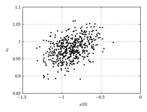
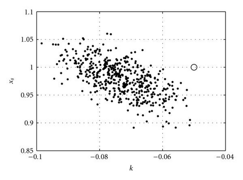
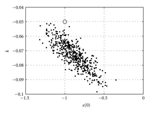
For the case where we have 6 observations at t = 2, 7, 12, 17, 22, and 27, with a random error of 0.01 (standard deviation), we have executed an ensemble experiment with 100 members to recover control. In this case, the condition number is 2.4 × 10³. Results are plotted three dimensionally and in two-dimensional planes in the space of control, that is, plots of correction in the xs/x(0), xs/k, and x(0)/k planes. Results are shown in Figure 2.
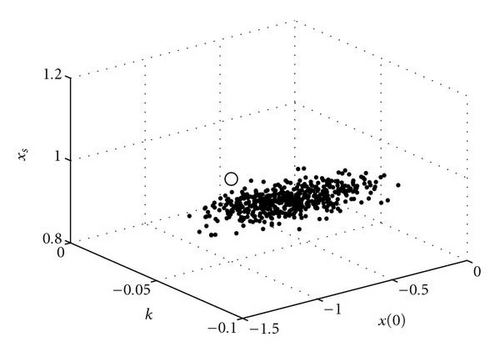
Details are in the caption following the image
Figure 2 (a) 3D clusterplot
3D cluster and its projections where corrections are computed using observations at the following times: t = 2, 7, 12, 17, 22, and 27. An ensemble of 100 members is used where the standard deviation of the observation noise is 0.01.
Details are in the caption following the image
Figure 2 (b) Cluster of corrections of x(0) versus k
3D cluster and its projections where corrections are computed using observations at the following times: t = 2, 7, 12, 17, 22, and 27. An ensemble of 100 members is used where the standard deviation of the observation noise is 0.01.
Details are in the caption following the image
Figure 2 (c) Cluster of corrections of x(0) versus xs
3D cluster and its projections where corrections are computed using observations at the following times: t = 2, 7, 12, 17, 22, and 27. An ensemble of 100 members is used where the standard deviation of the observation noise is 0.01.
Details are in the caption following the image
Figure 2 (d) Cluster of corrections of k versus xs
3D cluster and its projections where corrections are computed using observations at the following times: t = 2, 7, 12, 17, 22, and 27. An ensemble of 100 members is used where the standard deviation of the observation noise is 0.01.

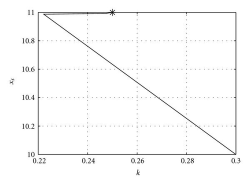
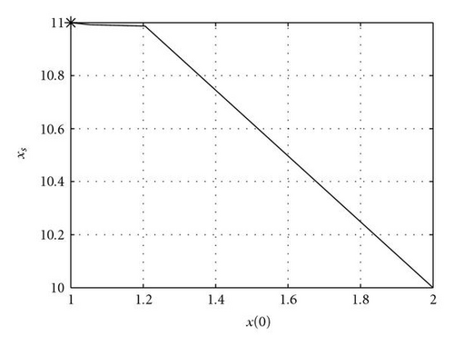
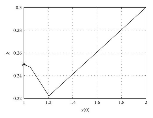
Finally, we explore the iterative process of finding corrections to control. Here, the results from the 1st iteration are used to find the new control vector. This vector is then used to make another forecast and find a new set of sensitivity functions. The error of the forecast is obtained, and along with the new sensitivity functions, a second correction to control is found, and so forth. For the experiment with 6 observations that has been discussed in the previous paragraph, we apply this iterative methodology. As can be seen in Figure 3, the correct value of control is found in 3 iterations.
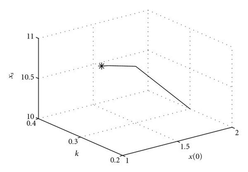
Details are in the caption following the image
Figure 3 (a) Iterative correction
An illustration of the progression of first-order iterative corrections using six observations at t = 2, 7, 12, 17, 22, and 27.
Details are in the caption following the image
Figure 3 (b) Projection onto x(0)-k plane
An illustration of the progression of first-order iterative corrections using six observations at t = 2, 7, 12, 17, 22, and 27.
Details are in the caption following the image
Figure 3 (c) Projection onto k-xs plane
An illustration of the progression of first-order iterative corrections using six observations at t = 2, 7, 12, 17, 22, and 27.
Details are in the caption following the image
Figure 3 (d) Projection on to x(0)-xs plane
An illustration of the progression of first-order iterative corrections using six observations at t = 2, 7, 12, 17, 22, and 27.

6. Concluding Remarks

The basic contributions of this paper may be stated as follows.

(1) While the 4D-Var has been the primary methodology for operational data assimilation in meteorology/oceanography (Lewis and Lakshmivarahan [11]), and while forward sensitivity has been a primary tool for reaction kinetics and chemistry (Rabitz et al. [1]) and air quality modeling (Russell et al. [3], to our knowledge these two methodologies have not been linked. We have now shown that the method of computing the gradient of J(c) by these two approaches exhibits a duality hitherto unknown.

(2) By treating the forward sensitivity problem as an inverse problem in data assimilation, we are able to understand the fine structure of the forecast error. This is not possible with the standard 4D-Var formulation using adjoint equations.

(3) While it is true that computation of the evolution of the forward sensitivity involves computational demands beyond those required for solving the adjoint equations in the standard 4D-Var methodology, there is a richness or augmentation to the information that comes with this added computational demand. In essence, it allows us to make judicious decisions on placement of observations through understanding of the time dependence of correction to control.

Acknowledgments

At an early stage of formulating our ideas on this method of data assimilation, Fedor Mesinger and Qin Xu offered advice and encouragement. Qin Xu and Jim Purser carefully checked the mathematical development, and suggestions from the following reviewers went far to improve the presentation: Yoshi Sasaki, Bill Stockwell, and anonymous formal reviewers of the manuscript. S. Lakshmivarahan’s work is supported in part by NSF EPSCoR RII Track 2 Grant 105-155900 and by NSF Grant 105-15400, and J. Lewis acknowledges the Office of Naval Research (ONR), Grant No. N00014-08-1-0451, for research support on this project.

    Appendices

    A. Dynamics of Evolution of Perturbations

    Let δc = (δxT(0), δαT) TRn × Rp be the perturbation in the control vector c and δx(t) the resulting perturbation in the state x(t) induced by the dynamics (1a) and (1b). Our goal is to derive the dynamics of evolution of δx(t).

    From first principles, the evolutionary dynamics of δx(t) are given by the variational equation (Hirsch et al. [12]) or the tangent linear model (Lewis et al. [7])
    (A.1)
    where the Jacobians A(t) and B(t) are given by
    (A.2)
    Define the integrating factor
    (A.3)
    premultiplying both sides of (A.1) by M−1(t, 0) and integrating, we get the solution of the linear nonhomogeneous and nonautonomous equation (A.1) as
    (A.4)
    where
    (A.5)
    From definitions (A.3)–(A.5), it can be verified that, for u < s < t,
    (A.6)
    We now consider two special cases.

    Case A. Let δα = 0, that is, the initial perturbations are confined only to the initial condition, x(0). Then setting B(t) ≡ 0, from (A.5) we see that L(t, 0) ≡ 0. From (A.4) we get

    (A.7)

    Case B. Let δx(0) = 0, that is, the initial perturbations are confined only to the parameter, α. Then setting A(t) ≡ 0, from (A.3), we see that M(t, s) ≡ I, the identity matrix. Now from (A.4) it follows that

    (A.8)

    B. Computation of Sensitivity Functions

    Let c = (c1, c2, …, cq) TRq, where x = x(t, c) = (x1(t, c), x2(t, c), …, xn(t, c)) TRn and h(x) = (h1(x), h2(x), …, hm(x)) TRm. Let a = (a1, a2, …, am) TRm and consider
    (B.9)
    By applying the standard chain rule it can be verified that the gradient ∇cϕ1(c) with respect to c is given by
    (B.10)
    where
    (B.11)
    is the Jacobian of h and
    (B.12)
    is the (Jacobian) sensitivity of the vector x with respect to c at time t.
    Now consider a quadratic form
    (B.13)
    where ARm×m is a symmetric and positive definite matrix.
    Then by the product rule
    (B.14)
    where b = Ah = a. By applying (B.10) to each of the two terms on the right side of (B.14), it follows that
    (B.15)
    Finally, if
    (B.16)
    then expand
    (B.17)
    since z does not depend on c, by using (B.10) and (B.15), we get
    (B.18)
    Define
    (B.19)
    then
    (B.20)
    That is, the gradient of Q with respect to c is the linear combination of the sensitivity vectors, that is, the columns of , where the coefficients in this linear combination are the elements of the vector ξ.

    C. Computation of ∇αJ in (27)

    Given η(ti), MT(ti, ti−1), LT(ti, ti−1) for 1 ≤ iN, the expression on the right-hand side of (27) can be efficiently computed as shown in Algorithm 1.

      Algorithm 1:
    • DO j = N to 1

    •  DO i = N to j

    • η(ti) = MT(tj, tj−1)η(ti)

    •  END

    • END

    • μ(1) = L(t1, 0)

    • DO i = 2 to N

    • μ(i) = μ(i − 1) + L(ti, ti−1)

    • END

    • Grad = 0

    • DO i = 1 to N

    • Grad = Grad + μ(i)η(ti)

    • END

    Then ∇αJ = − Grad. It is to be noticed that there is only matrix-vector multiplication involved in these operations and not matrix-matrix multiplication.

      The full text of this article hosted at iucr.org is unavailable due to technical difficulties.