Process Monitoring with Multivariate p-Control Chart

1. Introduction

In the modern industrial context, operators are usually interested in evaluating process quality. Assuming that the quality depends on several correlated quality characteristics, it is appropriate to use multivariate quality control methodology. If the quality characteristics are defined on nominal or ordinal scale, then the corresponding monitoring process is said to be a multivariate attribute process. For a general review of methods for monitoring multivariate attribute process see Topalidou and Psarakis [1]. Each item is inspected and classified as conforming or nonconforming, and different criteria for nonconforming classification may be used. For example, an item may be classified as absent, incidental, minor, or major defect, see Nelson [2]. Real example is shown in Taleb and Limam [3] and Taleb [4] where the porcelain industry items are classified as standard, second choice, third choice, or chipped.

In general, each item may be classified in (k + 1) ordered and mutually exclusive quality categories depending on the level of defect: the first category can be used to classify the conforming defect-free items, while the remaining k categories can be used to classify the nonconforming items in k distinct defect grades, with an increasing degree of nonconformity. In this case, the probabilistic model is the multinomial distribution, which is appropriate to define a statistical procedure to monitor this multivariate attribute process.

The most applied statistical method of monitoring the multinomial process is the chi-square control chart, originally proposed by Duncan [5]. This control chart is based on the chi-square sampling statistic to test the goodness of fit to the in control distribution and is a one-sided Shewhart-type control chart with only the upper approximate probabilistic control limit. The chi-square control chart is useful for identifying significant departures of almost one of the (k + 1) proportions from their in control values. The chart signals any changes in the quality target parameters, but it is unable to distinguish between increasing or decreasing levels of quality. If the chi-square sampling statistic plots out the upper control limit, then we may declare that the process is out of control, but cannot determine whether the defect proportion is increasing or not. To solve this limit, Marcucci [6] proposed a one-sided generalized p-chart, that is, specifically designed to indicate departures from the in control level only for the defect nonconforming proportions without considering the conforming proportion; but this chart is still one-sided and is designed to signal increases in the defect proportion and consequently identifies decreases in quality level only. Consequently, the chi-square control chart, proposed by Duncan [5], and the control chart, proposed by Marcucci [6], can be used only to identify process performance because they are able only to alert operators of any deterioration of the process so the potential damage can be alleviated or averted in time. From the management point of view, the ability to detect process improvements is very important since improvements can take place as a result of process stabilization, subprocess improvement, or learning effects. Continuous improvement of a high-quality process, although difficult and not straightforward, is an important issue to increase competition in the global market [7]. So in many manufacturing processes it is also becoming increasingly important to be able to detect moderate shifts in the performance of a process [8]. An example of complex process with very low fraction nonconforming is the manufacturing of integrated circuits; in this case, different defects can be observed [9], each of which can be categorized according to defectiveness grade. Therefore, in this perspective a useful quality control statistical method have to be able in evaluating whether the global quality level is increasing or decreasing. The need for innovating the statistical methodology for monitoring high quality processes has been stressed in Calvin [10], Bourke [8], Kaminsky et al. [11], Xie and Goh [12], Quesenberry [13], Xie and Goh [14], Xie et al. [7, 15], and Niaki and Abbasi [16].

So it is useful to define a two-sided control chart that uses, respectively, the upper control limit and the lower control limit to signal the deterioration or the improvement of the process quality. In the following, we define the sampling statistic that may be used as an index of the overall defectiveness level of the process and as a statistic necessary to determine a corresponding two-sided control chart with the approximate probabilistic control limits. In fact, the process is usually assumed to be capable if the proportion of nonconforming items is very small and remains low or declines over time. Therefore, because we have chosen to classify the nonconforming items into k different defect grades, the overall proportion of nonconforming items depends on the k categories, which are not necessarily independent. To get this purpose we propose (i) a normalized index that can be used to evaluate the overall defectiveness of the process, and (ii) a two-sided Shewhart-type multivariate control chart to monitor the overall defectiveness of nonconforming items. The corresponding sampling statistic is used to define the normalized index and the multivariate p-control chart. The paper is organized as follows: in Section 2 the overall defectiveness index is defined; in Section 3 a two-sided multivariate p-control chart with approximate probabilistic control limits is proposed; Section 4 presents some numerical examples useful for evaluating the performance of the chart in three different quality situations; the last section provides conclusions.

2. An Overall Defectiveness Index

For evaluating the overall defectiveness of the production, we draw from the process a sample of n items. Each sampling item may be classified only in one of the (k + 1) ordered and mutually exclusive categories of quality defects. Let D = (D₀, D₁, …, D_i, …, D_k) be the vector of the (k + 1) defect categories. The generic component D_i indicates the ith category of defect degree; D₀ is the free-defect category and D_k is the most serious category of defect degree. Since different defects bring to the process different losses of quality then, corresponding to the vector D, we can define a vector of weights that are numerical evaluations of the defect degree found in the product; these weights may be selected on the following: dysfunction, dissatisfaction, economical loss, increasing costs, or demerit caused by defect. For example, if the vector D has only five categories, like absent, minor, medium, major, and serious defect, then we may associate weight zero to the first category, weight one to the last category, and other weights, between zero and one, to the other categories. For example, assuming as criterium the dysfunction present into the item, if the weight is fixed to 0.20 then this means that this type of defect implies a 20% of dysfunction. If arbitrary weights are used then we have to transform these data in such a manner as to obtain constants between zero and one.

Items are classified in each of the (k + 1) quality defect categories. In this case the multivariate random variable X = (X₀, X₁, …, X_i, …, X_k) has a multinomial distribution with parameters n and probability vector p = (p₀, p₁, …, p_i, …, p_k), such that 0 ≤ p_i ≤ 1 and $$. Specifically, X_i is the number of items in the sample that are classified in the D_i defect category and p_i is the probability that an item may be classified in the D_i defect category. In the quality control procedure, p_i is the proportion of nonconforming items classified as defective in the ith class. Consequently, the multivariate random variable X has a multinomial random distribution with parameters (n, p), where n is the sample size and p the probability vector.

If the operator has chosen to assign the same weight to every class of defects, then an overall defectiveness index may be the overall proportion of nonconforming items in the process; indirectly, the operator can use this index as a measure of the process capability. The process will be considered capable when conforming proportion is very high. Instead, it is reasonable to think that the operator assigns different weights for every type of defect, because they cause, in the process, different grades of dysfunction, dissatisfaction, economical loss, or demerit. In this case, we have to consider accurately this differentiation of weights if we are interested in evaluating and monitoring the real overall level of defectiveness in the process. This approach for classification of defective items was used in Lu et al. [17], to design the multivariate np chart. Further, these types of problems, particularly in the case of a process with a very high quality level, are also investigated in Xie et al. [7]. Moreover in Cassady et al. [18], using a normal approximation of sampling statistics, this scheme of item classification was applied to determine a 3-level control chart.

The null hypothesis in (5) is verified if and only if all the null hypothesis in (6) are verified; so, in this case, it should be appropriate to use simultaneous inference procedure, see Miller [19].

Since we want to design a control chart with control limits such that the overall error rate is not much larger than the nominal level α, then in the following we have to consider only the simultaneous confidence procedures and compare them with the nonsimultaneous approach. Besides, simultaneous procedures are suitable to solve the identification problem in multivariate quality control [25].

3. A Two-Sided Multivariate p Control Chart

The proposed control chart signals the deterioration of the process when the sampling statistic is plotted out the UCL or the improvement of the process when the sampling statistic is plotted out the LCL. Analysis of the pattern of plotted statistics may be used to identify significant changes in the process parameters. We note that, for a specified vector d, the sampling statistic $$ increases when at least one of the nonconforming proportions p_i,  i = 1,2, …, k, increases and decreases otherwise. Hence the control chart is able also to test the global hypothesis in (6) and (11).

The proposed statistical procedure is conservative because the overall coverage probability inside the control limits is at least (1 − α) and therefore the level of significance is not larger than α. Consequently, the in control Average Run Length (ARL₀), that is, the average rate of false alarms, is expected to be larger than that of the chi-square control chart. Note that in the nonsimultaneous approach, the coverage probability inside the control limits is expected less than (1 − α) and for that reason the level of significance is larger than α. Consequently the in control ARL₀ is expected to be smaller than that of the chi-square control chart. Nevertheless, the operator is more interested in evaluating the performance of control charts evaluating the out of control ARL₁, that is the average correct alarm rate to signal a true change.

4. Numerical Simulations

In this section, the performance of the control chart will be evaluated using three different cases of overall quality level: a low, high, and very high quality process. In particular, for the fixed sample size n and significance level α, fixed at 0.0027, the influence of the parameter k on the performance of the control chart will be evaluated through numerical simulation. Furthermore, we propose comparisons of performance of the control chart, designed by (a) simultaneous confidence interval based on Šidák’s inequality, (b) upper and lower quantiles estimated using empirical cumulative distribution function, and (c) nonsimultaneous confidence interval.

4.1. Example One: Low-Quality Level

A first example is based on real data reported in Taleb and Limam [3] about the production of porcelain. The items are classified by experts, with respect to quality, into four defect categories: standard, second choice, third choice, and chipped. In this case, the loss of quality may be evaluated in terms of economical loss; in fact, an item classified as standard or defect-free can be sold at the standard price, the second and third choice items sold at lower prices, while the chipped items cannot be sold at all. The following hypotheses, about the defect proportions in vector p, are used:

$$ ()

$$ ()

$$ ()

The in-control process (19) has a low-quality level because the proportion of defect-free items is fixed at 0.65. The hypothesis (20) indicates a deterioration in process since the maximum defect category is increased to 0.098; by contrast, hypothesis (21) indicates an improvement in process since the second and fourth defect categories are decreased, respectively, to 0.11 and 0.0204.

Usually, the operator is interested in identifying a deterioration in process and considers only the null hypothesis to choose the size of samples, but in our approach we want to develop a procedure that will also be able to identify an improvement in process. Therefore, for defining the appropriate sample size we have to consider the minimum proportion indicated in the process-improvement hypothesis. In this first example the minimum proportion is 0.0204; then by Cochran’s rule we have to take a sample of size n = 250.

For numerical evaluations we have simulated samples from multinomial processes with parameters n and p, respectively, defined in (19), (20), and (21). Using a random number generation procedure [28], for every hypothesis we have (i) simulated 10000 samples of size n = 250, (ii) calculated the sampling statistics $$, and (iii) plotted it on the multivariate p control chart with control limits designed on the in-control process hypothesis. Only 110 values of 30000 simulated samples are plotted in the graphical representations of control charts, see Figures 1, 2, and 3; specifically, the first 50 values are taken from an in-control process, the next 30 values are taken from a deteriorated process and the last 30 values are taken from an improved process.

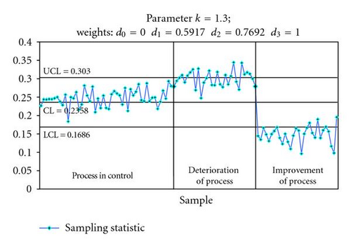
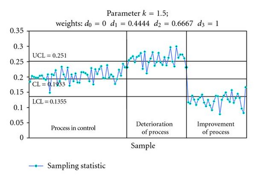
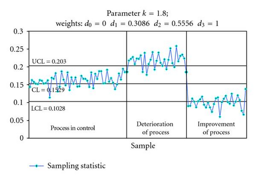
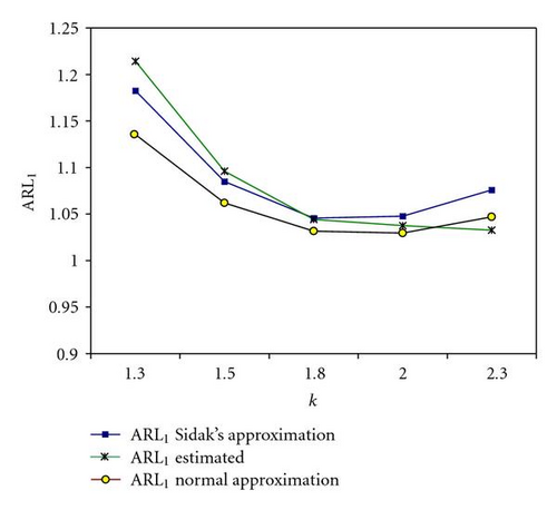
We note that if the parameter k, that is, chosen is small, near one, then the operator considers the defect categories similar in terms of loss of quality; instead, if the operator considers the highest categories more important than the lowest (in terms of loss of quality inducted in the process), then a higher parameter k has to be selected. We may note easily, from analysis of Figures 1–3, that the performance of control chart changes in conjunction with the value of parameter k. So we want to evaluate, using simulated data, the ARL₁ in function of different values of parameter k. In particular, we estimate the two one-sided ARL₁: ARL₁(upper) and ARL₁(lower). The ARL₁(upper) indicates the control chart’s ability to identify correctly only deteriorations in the process; while ARL₁(lower) evaluates the control chart’s ability to identify significant improvements in process. Combining the two one-sided ARL₁ we can estimate the ARL₁. The ARL₁ curves in function of the parameter k are shown in Figure 4. Figure 4 shows that ARL₁(upper) and ARL₁(lower) are, respectively, decreasing and increasing values of parameter k. Also, for comparison purposes of the performance of the control chart we have estimated the values of ARL for charts with control limits determined by (a) the simultaneous confidence interval based on Šidák’s inequality, (b) the quantiles q_0.00135 and q_0.99865, estimated by the empirical cumulative distribution function, and (c) the non simultaneous confidence interval. Values of ARL are reported in Table 1 and graphical comparisons in Figure 5.

Table 1. ARL comparisons (example one).

	ARL for chart with simultaneous				ARL for chart with exact				ARL for chart with nonsimultaneous
	Šidák′s approximation control limits				estimated control limits				approximation control limits
k	ARL0	ARL1	ARL1	ARL1	ARL0	ARL1	ARL1	ARL1	ARL0	ARL1	ARL1	ARL1
		upper	lower			upper	lower			upper	lower
k = 1.3	555	2.855	1.063	1.959	370	2.610	1.039	1.824	270	2.377	1.037	1.707
k = 1.5	417	1.963	1.118	1.541	370	2.109	1.073	1.591	286	1.734	1.077	1.406
k = 1.8	500	1.518	1.291	1.405	370	1.583	1.154	1.369	256	1.392	1.194	1.293
k = 2	555	1.406	1.505	1.456	370	1.440	1.231	1.336	303	1.313	1.347	1.330
k = 2.3	555	1.311	1.959	1.635	370	1.344	1.432	1.388	333	1.239	1.639	1.439

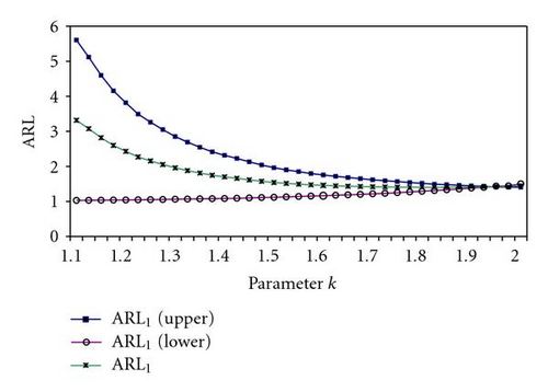
If we consider the results in Table 1 we have to conclude, since ARL₁(lower) < ARL₁(upper), that the proposed control chart is better to identify process improvement for k ≤ 1.8. The same evidence is obtained from the analysis of the ARL₁ curves in Figure 4. In fact, the distance between the ARL₁(upper) curve and the ARL₁(lower) curve is high for small values of k and small for large values. However, the result is valid from operator’s perspective. Note that it is reasonable to assume value of k ≤ 1.5; in fact, in this case the operator assumes that each class of defect, in terms of defectiveness, is more important of 50% respect to the previous class.

Besides, to exemplify the methods for calculating the ARL reported in Table 1 and Figure 4, consider the case when the operator uses the control chart with simultaneous Šidák′s approximation control limits, with k = 1.3. One thousand simulations have been carried out. Each experiment consisted in the generation of 10000 observations from a multinomial distribution with parameters n = 250 and probability vector defined in (19); that is, when the process is in control. For each experiment the Run Length in control (RL₀) has been calculated; that is, the number of observations where the sampling statistic defined in (2) assumes a value outside the control limits, identifying a false alarm. Then to estimate the ARL₀ the mean of the 1000 RL₀ simulation values has been calculated. Under the assumption of process in control the mean of the 1000 RL₀ was equal to 18. The false-alarm probability α is obtained by the ratio between the mean of RL₀ and the sample size; α = 18/10000 = 0.0018; therefore ARL₀ = 1/α = 555. Instead, using 1000 of simulations, each of which consists in 10000 observations from a multinomial distribution with parameters n = 250 and probability vector defined in (20); that is, when the process is out control. For each experiment the Run Length out of control (RL₁) has been calculated; that is, the number of observations where the sampling statistic defined in (2) assumes a value outside the control limits, identifying a really correct alarm. To estimate ARL₁ then the mean of the 1000 RL₁ simulation values has been calculated. Under the assumption of process out control the mean of the 1000 RL₁ was equal to 3503. The correct-alarm probability (1 − β) is obtained by the ratio between the mean of the RL₁ and the sample size; (1 − β) = 3503/10000 = 0.3503; therefore ARL₁ = 1/(1 − β) = 2.855.

4.2. Example Two: High-Quality Level

A second example considers a process with a higher level of quality than that considered in case one; in fact, the defect-free proportion, that is, chosen is equal to 0.83. The following hypotheses, about the defect proportions in vector p, are used:

$$ ()

$$ ()

$$ ()

As in the first example, the hypothesis (23) indicates a deterioration in process and the hypothesis (24) indicates an improvement in process. Since the minimum proportion is 0.0101, then in accordance with Cochran’s rule we have to take a sample of size n = 500. The same simulation procedure described in example one is used. From Figures 6, 7, and 8 the performance of the control chart evidently depends on the value of parameter k. For the hypothesis under investigation, that is, to consider the process at a high level of quality, the chart seems to perform better. In fact, comparing ARL₁ curves in Figures 4 and 9 and data in Tables 1 and 2, we can conclude that the control chart performs better at a high level of quality than at a low level of quality, particularly when the statistical procedure is used to identify improvement in the process.

Table 2. ARL comparisons (example two).

	ARL for chart with Šidák′s				ARL for chart with exact				ARL for chart with normal
	approximation control limits				estimated control limits				approximation control limits
k	ARL0	ARL1	ARL1	ARL1	ARL0	ARL1	ARL1	ARL1	ARL0	ARL1	ARL1	ARL1
		upper	lower			upper	lower			upper	lower
k = 1.3	455	1.365	1.000	1.183	370	1.428	1.00000	1.214	256	1.271	1.000	1.136
k = 1.5	455	1.169	1.001	1.085	370	1.192	1.00020	1.096	256	1.124	1.000	1.062
k = 1.8	435	1.076	1.015	1.046	370	1.085	1.00370	1.044	270	1.056	1.007	1.032
k = 2	526	1.056	1.04	1.048	370	1.065	1.01060	1.038	312	1.037	1.022	1.030
k = 2.3	625	1.037	1.115	1.076	370	1.037	1.02838	1.033	294	1.024	1.070	1.047

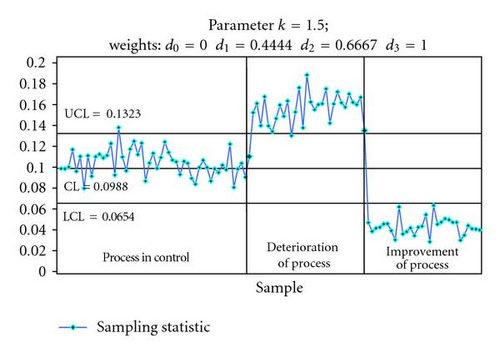
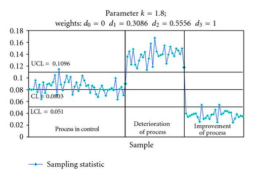
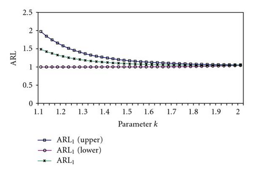
Table 2 and Figure 10 report for example two, the values of ARL for procedures based (a) on Šidák’s inequality, (b) on empirical estimation and (c) on normal approximation.

If we consider the results in Table 2 we conclude that, as in the example one, since ARL₁(lower) < ARL₁(upper), then the proposed control chart is better to identify process improvement for k ≤ 2. The same evidence is obtained from the analysis of the ARL₁ curves in Figure 9. In fact, the distance between the ARL₁(upper) curve and the ARL₁(lower) curve is high for small values of k and small for large values. The results, considering data in Table 2 and Figure 9, obtained in the case of high-quality level, are better than that obtained in the case of low-quality level.

4.3. Example Three: Very High-Quality Level

A third example considers a process with a much higher level of quality than that considered in cases one and two; in fact, the defect-free proportion, that is, chosen is equal to 0.99 and the maximum defective proportion is 0.001, that is, 1000 ppm. This level of quality will be classified as very high. The following hypotheses, regarding the defect proportions in vector p, are used to evaluate the performance of the multivariate p control chart:  

$$ ()

$$ ()

$$ ()

The hypothesis (26) indicates a deterioration in process and the hypothesis (27) indicates an improvement in process, since the minimum proportion is 0.001, then in accordance with Cochran’s rule we have to take a sample of size n = 5000. The same simulation procedure described in example one is used. As in the previous examples, the performance of the control chart evidently depends on the value of parameter k. For the hypothesis under investigation, considering the ARL₁ values, the chart works much better than it does at the low and high quality levels. In fact, the ARL₁ in the example process with very high-quality level is always smaller than that in the example processes with high or low quality level. This indicates that our approach is more appropriate in the case of a process with a very high level of quality (see Figures 11, 12, 13 and 14).

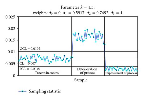
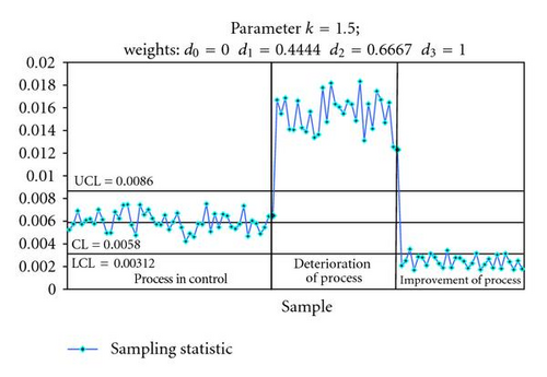
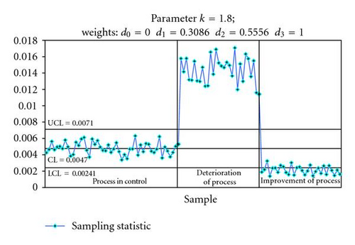
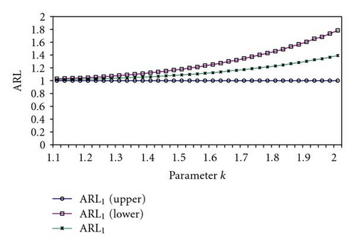
Table 3 and Figure 15 report the values of ARL in the function of parameter k.

Table 3. ARL comparisons (example three).

	ARL for chart with Šidák′s				ARL for chart with exact				ARL for chart with normal
	approximation control limits				estimated control limits				approximation control limits
k	ARL0	ARL1	ARL1	ARL1	ARL0	ARL1	ARL1	ARL1	ARL0	ARL1	ARL1	ARL1
		upper	lower			upper	lower			upper	lower
k = 1.3	1250	1.000	1.080	1.040	370	1.000	1.034	1.017	385	1.000	1.042	1.021
k = 1.5	909	1.000	1.179	1.089	370	1.000	1.085	1.042	400	1.000	1.109	1.055
k = 1.8	769	1.000	1.460	1.230	370	1.000	1.211	1.106	526	1.000	1.302	1.151
k = 2	769	1.000	1.783	1.392	370	1.000	1.378	1.189	526	1.000	1.502	1.251
k = 2.3	909	1.000	2.539	1.770	370	1.000	1.586	1.293	455	1.000	1.999	1.500

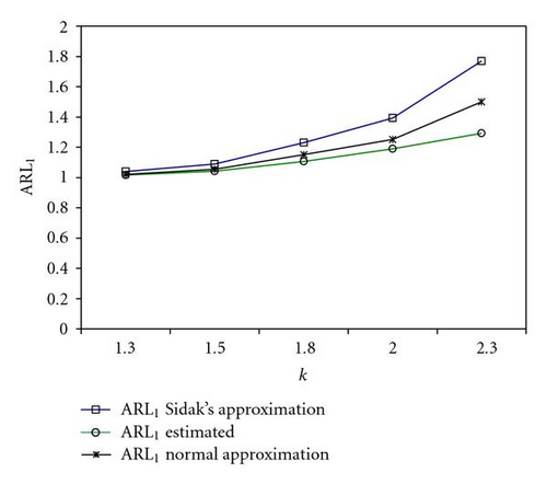
The comparisons of the ARL, reported in the Tables 1–3 point out that (i) ARL₁ is always better for the control chart with non simultaneous approximation control limits; (ii) ARL₀ is always better for the control chart with simultaneous Šidák′s approximation control limits; that is, the false alarm probability is always smaller in the simultaneous approach respect to the nonsimultaneous approach. In general, a good multiattribute quality control procedure is one that provides a method for identifying which subset of the classes of defects are responsible when the process is determined to be out of control. The control chart proposed in this paper and based on simultaneous confidence intervals meets this criterium. On the contrary the non simultaneous approach is not able to solve the identification problem (see [25]).

5. Conclusions

In this article an index of weighted overall defectiveness of the process and a two-sided multivariate p control chart to monitoring the quality of the process are defined. Using simultaneous confidence interval, based on the Šidák′s inequality, approximate control limits are determined. Specifically, the control chart is designed to identify changes in any of the defective class proportions and, differently of the one-sided chi-square control chart, is able to identify process deterioration or process improvement. Besides, if the control chart signals an out of control situation, then, estimating simultaneous confidence intervals for every parameters, the identification problem can be solved.

The sampling statistic used to estimate the overall defectiveness of the process and to design the corresponding control chart is function of the weights associated to the vector of quality defect categories. Therefore, the performance of the control chart is influenced by these values. In this paper we propose to use weights that are in terms of the geometric progression; the parameter k is the common ratio of thegeometric sequence. The performance of the control chart has been evaluated using simulated data from multinomial process in three different hypotheses: low, high, and very high quality level of the process. Properties of the ARL are examined and investigated by numerical simulations in function of different values of the parameter k. Some numerical comparisons, in terms of corresponding ARL, for control charts with different control limits, are proposed. The control chart is more effective in presence of very high quality level, specifically, in identifying improvement of the process.

An interesting methodological development is possible considering the multivariate binomial distribution as appropriate probabilistic model to monitor the process quality degree, because it is a more general distribution which contains the one used in this paper.