Particle Swarm Optimization for Multimodal Functions: A Clustering Approach
Abstract
The particle swarm optimization (PSO) algorithm is designed to find a single optimal solution and needs some modifications to be able to locate multiple optima on a multimodal function. In parallel with evolutionary computation algorithms, these modifications can be grouped in the framework of niching. In this work, we present a new approach to niching in PSO based on clustering particles to identify niches. The neighborhood structure, on which particles rely for communication, is exploited together with the niche information to locate multiple optima in parallel. Our approach was implemented in the k-means-based PSO (kPSO), which employs the standard k-means clustering algorithm, improved with a mechanism to adaptively identify the number of clusters. kPSO proved to be a competitive solution when compared with other existing algorithms, since it showed better performance on a benchmark set of multimodal functions.
1. Introduction
The design of optimization algorithms is usually targeted to the goal of finding a single optimal solution for a given problem. However, in many situations, this can be less than ideal. Some problems have multiple possible solutions which are optimal according to the chosen criterion. In these cases, an optimization algorithm should ideally find all the optimal solutions; then, these solutions can be used in many different ways, depending on the application field: a specific solution can be selected from the set using additional criteria, different solutions can be preferred in different situations, or a combination of multiple solutions can be built.
In general, optimization problems are formalized identifying the function to optimize. When such a function presents multiple global optima, or local optima whose values are very close to the global one, it is said to be multimodal. In dealing with multimodal functions, the behavior of a standard optimization algorithm may be less than ideal. In some cases, in fact, an algorithm designed to look for a single optimum would arbitrarily pick just one of the optimal solutions, or it could even be misled by the presence of more than a single optimum and fail to converge (e.g., some genetic algorithms [1]). Thus, it is necessary either to design specific algorithms, or to modify the generic ones in order to optimize multimodal functions.
The latter approach has been taken, for example, in the field of evolutionary computation. Optimization algorithms based on the principles of Darwinian evolution have been modified introducing the concept of niching. In an environment with limited resources, the evolutionary process leads to the emergence of different species, which tend to exploit different niches. When applied to a search algorithm, niching allows it to divide the space in different areas and search them in parallel.
In this study we will focus on particle swarm optimization (PSO), a class of optimization algorithms which is strongly tied to evolutionary computation. We will examine how niching techniques can be introduced in the particle swarm algorithm, observing similarities and differences in relation to evolutionary algorithms. After discussing previous approaches towards a niching particle swarm, we will introduce a new approach based on clustering. Moreover, we will produce an implementation of the clustering approach, kPSO, which uses the k-means clustering algorithm to identify niches in the population.
The paper starts with a brief introduction to the PSO algorithm, which focuses on pointing out the importance of the neighborhood structure of the swarm (Section 2). Then, in Section 3, the topics of multimodal function optimization and niching are discussed and previous applications of niching in the context of PSO are presented. Section 4 is dedicated to a detailed introduction of our clustering approach to niching and its first implementation, kPSO. In Section 5, we show the results obtained by the new algorithm from the experiments set up to compare its performance to those of other PSO niching algorithms. Finally, in Section 6, conclusions are drawn from the current results, and future research directions are pointed out.
2. Particle Swarm Optimization
PSO is a quite recent algorithm which can be used to find optimal (or near optimal) solutions to numerical and combinatorial problems. It is easily implemented and has proven both very effective and quick when applied to a diverse set of optimization problems.
PSO was originally developed by Kennedy and Eberhart in 1995 [2], taking inspiration both in the related field of evolutionary algorithms and in artificial life methodologies. In fact, the origins of particle swarm algorithms are strongly tied to the artificial life theory of bird flocking, fish schooling, and swarming; however, PSO is also considered a kind of evolutionary algorithm, with many similarities in particular with genetic algorithms and evolutionary programming [3].
The PSO algorithm simulates the flight of a population of particles (the swarm) in a multidimensional space, where each particle represents a candidate solution to the optimization problem. Particles′ flight is influenced by the best positions previously found by themselves and the other particles. The effect is that particles generally tend towards optimal positions, while still searching a wide area around them.
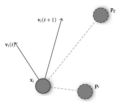
In this way, the likelihood of particles leaving the search space is reduced, although indirectly, by limiting the maximum distance a particle will cover in a single step.
An essential feature of the PSO algorithm is the way in which the local and global best positions, pi and pg, and their respective acceleration coefficients, are involved in velocity updates. Conceptually, pi (also known as pbest) represents the particle′s autobiographical memory, that is, its own previous experience, and the velocity adjustment associated with it is a kind of simple nostalgia, as it leads the particle to return to the position where it obtained its best evaluation. On the other hand, pg (gbest) is a sort of group knowledge, a common standard which every single particle seeks to attain.
The overall effect is such that when particles find a good position, they begin to look nearby for even better solutions, but, on the other hand, they continue to explore a wider area, likely avoiding premature convergence on local optima and realizing a good balance between exploration of the whole search space and exploitation of known good areas.
2.1. Neighborhood Structure
So far, we have described swarms in which particles had access to the accumulated knowledge of the whole population, as they were attracted by the global best solution, gbest. However, this is not by far the only possible choice. More generally, in fact, we can have particles influenced by the best solutions found in their neighborhood, that is a specific subset of the population. The mathematical relation which defines the neighbors of each particle constitutes the neighborhood topology and can be described by a—typically undirected—graph in which each particle is a vertex and its neighborhood relations are represented by adjacent edges (see Figure 2).

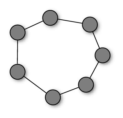
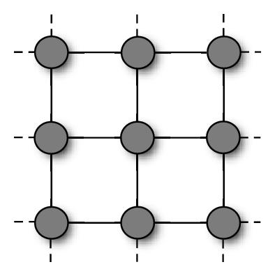
The role of the neighborhood topology is to regulate the information flow among particles. In the PSO algorithm, particles communicate by sharing high-fitness solutions they previously located with their neighbors. Thus, the communication takes place along the channels defined by the neighborhood structure. On a dense topology, particles would have many neighbors, so the knowledge of a good position would be rapidly shared. Conversely, on more sparse structures, the information would spread at a slower rate.
The swarm in which a global best position is shared among all particles, also called the gbest particle swarm, is thus the special case whose topology is a fully connected graph, so that each particle′s neighborhood is the whole swarm (Figure 2(a)). At the other extreme is the cognition-only model [5], in which we have no edges in the graph: a particle′s neighborhood is thus empty. However, in this way we would no longer have a swarm, but a group of isolated particles wandering around with no interactions.
A more common variation is the so-called lbest particle swarm, in which particles are modeled to have only local interactions [6] (Figure 2(b)). The topology structure is a regular ring lattice with k edges per vertex, so that each particle is influenced by k neighbors. A commonly used lbest case is k = 2, resulting in individuals affected by only their immediately adjacent neighbors. In such a swarm, it might be the case that a segment of the population converges on a local optimum, while another converges on a different optimum or keeps searching. However, if an optimum is really the best found by any part of the population, its influence slowly propagates along the ring, and eventually all the particles will be pulled towards it.
First experiments with the particle swarm used mainly the gbest and lbest versions, with the first generally thought to perform better in most cases. Since then, many other topologies have been proposed and studied. Suganthan [7], for example, proposed a swarm in which neighborhood relations extend over time, in order to increase cooperation towards the end of a run.
In [8], probably the first systematic study on the performances of different topologies, Kennedy and Mendes recommended the Von Neumann′s architecture (Figure 2(c)), in which a particle′s neighbors are above, below, and on each side on a two-dimensional lattice, to be the most promising one.
3. Multimodal Function Optimization
A function is multimodal if it has more than one optimum. However, it may have either a single global optimum or more than one. When trying to optimize a multimodal function, very different problems arise in each of these cases. Optimization algorithms applied to functions with a single global optimum and many local optima usually have the goal of locating the one global optimum. Thus, their main problem is to avoid deception by the other optima of the multimodal function, which would otherwise result in premature convergence to a suboptimal solution. In the other case, when the function has many optima with the same value, the goal of an optimization algorithm may be to locate all of them.
Most optimization techniques are designed to deal with multimodal functions of the first kind. They usually assume that there exists only a single best solution in the search space, and they put efforts in isolating it from other spurious solutions.
The situation is much different when dealing with functions with more than a single global optimum. In this case, standard techniques will usually either favor a single solution, or get confused by the multiple possible solutions and fail to converge to a single one. Therefore, specific algorithms need to be employed or the standard ones need to be modified to be more effective on multimodal functions.
3.1. Niching
In the field of evolutionary algorithms, multimodal functions are dealt with by introducing the concept of niching. Niching techniques are modeled after a phenomenon in nature where animal species specialize in exploiting different kinds of resources, resulting in several species coexisting in the same environment [1]. The introduction of this specialization, or niching, into a search algorithm allows it to divide the space in different areas and search them in parallel. The technique has proven useful when the problem domain includes multiple global and local deceptive optimal solutions.
Given the similarities between the evolutionary and the particle swarm approaches, it is natural to consider a parallel development of niching for PSO. There are, however, some peculiarities of the particle swarm approach which need to be considered.
Niching methods for genetic algorithms modify the way individuals interact with each other, in order to let them specialize on different areas of the search space, instead of converging on a single one. In the evolutionary approach individuals interact rather indirectly, as a combined effect of the selection and recombination operators. In fact, the various niching methods use different approaches, depending on the specific interaction factor they choose to modify.
The situation with the PSO algorithm is rather different. The particles in the swarm interact in a much more straightforward way than evolving individuals. In fact, the interaction is implemented by sharing knowledge of the search space with neighbor particles. Thus, the neighborhood structure of the swarm is probably the single most relevant aspect to consider in our analysis.
Let us consider for example the gbest swarm, that is a PSO in its simplest form. The gbest topology let particles interact with the whole swarm. As we have seen in the previous section, this provides for very quick convergence towards a good region of the space, which often is identified early in the search process. On a function with multiple global optima, this approach most often will simply converge on one of the optima and ignore the others.
Conversely, neighborhood topologies more sparsely connected lead to very different outcomes. A good example is the lbest topology, where particles have a very small neighborhood. In this case, the population tends to split into small groups which explore independently the search space. Thus, they can actually locate different optima at the same time, resulting in a sort of implicit niching capability. However, since the neighborhoods in the lbest swarm overlap, in many cases particles end up converging on the same optimum nonetheless. In the end, the implicit niching performed by the swarm relies too much upon random events during the running of the algorithm to be an efficient niching approach.
Thus, as pointed out by Engelbrecht et al. [9], the standard PSO must be modified to allow the efficient location of multiple solutions. Notwithstanding the differences between the approaches we will discuss for the particle swarm, with respect to the evolutionary ones, we will still refer to them as niching strategies.
3.1.1. Objective Function Stretching
Objective function stretching, introduced by Parsopoulos et al. [10, 11], was among the first strategies to modify the particle swarm algorithm to deal with functions with multiple optima. Specifically, the goal of the authors was to overcome the limitations of PSO caused by premature convergence to a local solution. The stretching approach operates on the fitness landscape, adapting it to remove local optima. Considering a minimization problem, when the swarm converges on a—possibly local—minimum, the fitness of that position is stretched so that it becomes a local maximum. In this way, successive iterations of the PSO algorithm will focus on other areas of the search space, leading to the identification of other solutions.
In [12], Parsopoulos and Vrahatis further developed the same technique to use it as a sequential niching approach. Likewise other sequential niching approaches, the stretching technique has some advantages, but critical issues. It requires no modifications of the underlying PSO algorithm and actually shows good performances on many multimodal functions. However, the effectiveness of the stretching transformation is not uniform on every function. In fact, in some cases it can introduce false minima, which render this method unreliable [13].
3.1.2. NichePSO
In 2002, Brits introduced the nbest PSO, reportedly the first technique to achieve a parallel niching effect in a particle swarm [14]. The nbest PSO was in particular aimed at locating multiple solutions to a system of equations, and used local neighborhoods determined by spatial proximity.
The same authors subsequently proposed a new approach which used subswarms to locate multiple solutions to multimodal function optimization problems: NichePSO [15]. NichePSO maintains a main swarm which can generate a subswarm each time a possible niche is identified. The main swarm is trained using the cognition-only model [5], which updates the velocities of particles considering only their personal best position. Since no social component is involved, each particle will perform a local search. On the other hand, the subswarms are trained using the GCPSO algorithm [16], which ensures convergence to a local optimum.
Niches in the fitness landscape are identified by monitoring changes in the fitness of particles. Specifically, a new subswarm is created when the fitness of a particle shows very little change over a fixed number of iterations. NichePSO has some rules to decide the absorption of particles into a subswarm, and the merging of two subswarms, which basically depends on the measure of the subswarm radius Rj.
This approach was compared empirically and shown to outperform two niching genetic algorithms—sequential niching [17] and deterministic crowding [1]—on a set of benchmark multimodal function optimization problems [18].
3.1.3. Parallel Vector-Based PSO
Schoeman and Engelbrecht proposed a different niching approach in [19], and implemented it in the vector-based PSO (VPSO). Their approach considered the two vector components of the velocity update formula in (1), which point, respectively, towards the particle′s best position and the neighborhood best. When these two vectors point roughly towards the same direction (and thus have a positive dot product), the particle will modify its trajectory towards the neighborhood best, otherwise (negative dot product), it will probably head for another optimal solution. Niches are identified according to this criterion. In fact, once the dot product is determined for each particle in the swarm, the niche radius can be defined as the distance from the neighborhood best of the closest particle with a negative dot product.
The original VPSO algorithm identified and exploited niches in a sequential way, starting from the global best and then repeating the procedure for the particles outside its niche. In [20], the same authors developed the parallel vector-based PSO (PVPSO), a more efficient version, based on the same principles, but which followed a parallel approach. In this case, the different niches are identified and maintained in parallel, with the introduction of a special procedure which can merge two niches when they become closer than a specified threshold ϵ.
The vector-based approach has the appealing property of identifying niches by using operations on vectors which are inherent to the particle swarm algorithm. Thus, it provides an elegant way to build a particle swam for multimodal function optimization. However, when it was tested on common benchmark functions, the results showed that its performances were lower than those of other approaches, such as the NichePSO.
3.1.4. Species-Based PSO
Another niching version of the particle swarm algorithm, the species-based PSO (SPSO) was proposed by Li [21]. The approach was the adaptation to the particle swarm of the species conserving genetic algorithm [22], of whom Li himself had been among the proponents. In particular, SPSO adopted the same procedure for determining the species seeds, which identify the niches in the population. This procedure is in fact essentially analogous to the clearing procedure proposed by Petrowski [23].
Once the species seeds have been identified, all the other particles are assigned to the niche formed by the closest seed, and the neighborhood structure is adapted to reflect the division in niches. In fact, each species seed would serve as the nbest for all the other particles in its niche.
The SPSO niching approach can dynamically identify the number of niches in the fitness landscape, and also proved to be suitable for the application on dynamics environments [24]. However, it still requires a radius parameter σ to determine the extension of the niches. Moreover, it implicitly assumes that all the niches have roughly the same extension.
3.1.5. Adaptive Niching PSO
In [25], Bird and Li developed a new algorithm which could adaptively determine the main niching parameters: the adaptive niching PSO (ANPSO).
This value is then used to determine the formation of niches. In fact, ANPSO keeps track of the minimum distance between particles over a number of steps. At each iteration, the graph 𝒢 with particles as nodes is considered, and an edge is added between every pair of particles which have been closer than r in the last 2 steps. Niches are formed from the connected subgraphs of 𝒢, while all the particles which end up with no edges remain outside any niches. As it can be seen from (6), the computational cost of the niche formation procedure is O(N2) with respect to distance calculations, which is quite expensive in comparison to other techniques. ANPSO executes a particle swarm simulation with constriction factor, but redefines the neighborhood topology at each step. In fact, once it determines the niches, it uses a gbest topology for each niche, and a von Neumann topology for unniched particles. In this way, the particles which have formed a niche will tend to perform a local search around an optimum, while the others will continue searching the whole space.
4. Clustering Particles
The particle swarm optimization algorithm has many points in common with evolutionary algorithms. Certainly enough to allow the concept of niching, originated in the evolutionary framework, to be applied to it. However, some peculiarities of PSO must be taken into account. In PSO, there is no selection mechanism: all interactions among particles take place along the neighborhood structure. Thus a niching mechanism should operate directly or indirectly on it, modifying neighborhood relationships among particles. Another aspect by which PSO differs from the evolutionary approach is the memory particles keep of their previous best positions. This information can definitely be exploited in the discovery of niches.
We discussed in the previous section the implicit niching capabilities which the PSO enjoys. Though they are not sufficient to provide for an effective method for the location of multiple optima, they are considered a good starting point to build on. As stated by Kennedy and Eberhart:
After a few iterations, particles in the particle swarm are seen to cluster in one or several regions of the search space. These clusters indicate the presence of optima, where individuals′ relatively good performances have caused them to attract their neighbors, who in moving towards the optimal regions improved their own performances, attracting their neighbors, and so on [26].
In fact, the tendency of particles to group near the optima of the function is balanced in the end by the social influence of the particle which has found the best position. Depending on the specific neighborhood topology, this influence will extend to the other particles in the swarm at different rates. However, since the graph representing the neighborhood relationship is in general a connected graph, eventually all particles will tend to be attracted towards a single position.
The basic idea behind our approach is to dynamically adapt the neighborhood structure in order to form different niches in the swarm. This is accomplished by applying a standard clustering algorithm to identify niches and then restricting the neighborhood of each particle to the other particles in the same cluster. In this way each cluster of particles tends to perform a local search in the function domain and to locate a different optimum.
4.1. Stereotyping
The use of clustering on the particles of a swarm is not new. In [27], Kennedy introduced the concept of stereotyping and discussed its impact on the performance of the PSO algorithm. A stereotype is an individual or the idealization of an individual which represents the norm of a group. The algorithm presented by Kennedy used clustering to identify different groups in the swarm and defined the centroid of each cluster as the stereotype which the particles in that cluster would look at.
Kennedy′s study was related to the social metaphor underlying the particle swarm. In the standard PSO, particles are attracted towards their personal best position and the best position among their neighbors. This attraction simulated the tendency to follow the best individual of a group. The application of stereotyping shifted this attraction from the best individual to a statistical prototype (the centroid of each cluster).
Stereotypes were identified by a cluster analysis on the particles′ previous best positions, performed with a version of the k-means clustering algorithm. The experiments on stereotyping were aimed at studying the swarm behavior when the cluster center was used in place of the individual best or of the neighborhood best in the velocity update formula. Results showed that substituting the individual previous best with its cluster′s center gave it some advantage, while substituting the neighborhood best with the respective centroid did not. A possible explanation is that using a stereotype in place of an individual is on average a quite good choice, while substituting the best individual with the stereotype will in general lower its fitness.
In the end, the use of clustering for a stereotyping approach brought some useful insights in the study of the particle swarm. However, its goals were completely unrelated to niching. In the following, we will introduce a new variation of the particle swarm technique which uses a very similar clustering procedure, but focuses on the identification of niches.
4.2. k-Means Particle Swarm Optimization
The algorithm we developed is the k-means particle swarm optimization (kPSO), the first version of which was introduced in [28]. It provides a basic implementation of our clustering approach to niching. In particular, we employed the standard k-means algorithm, which is probably the best-known partitional clustering algorithm [29, 30], to cluster particles according to their pbest, the previous best position. k-means is a very simple algorithm and, as we have just seen, it had already been applied by Kennedy to cluster particles in a swarm in his research on stereotyping.
kPSO uses the clusters of particles to modify the neighborhood topology so that each particle can communicate only with particles in the same cluster. Therefore, the swarm turns in a collection of subswarms which tend to explore different regions of the search space. Since our goal is that the subswarms perform a rather local search, each of them uses a gbest topology, with all the particles in a cluster connected to each other.
Clustering is performed after the swarm random initialization and then repeated at regular intervals during the swarm simulation. Between two clustering applications the swarm (or more precisely, the subswarms corresponding to the various clusters) follows its (their) normal dynamics. In fact, the multiple applications of the clustering algorithm are meant to keep track of the swarm dynamics: particles in different clusters at early stages of the simulation can end up in the same cluster as they move towards the same local optimum or, in contrast, a single cluster can be split into two as some of its particles fly towards a different optimum.
A relevant difference between our approach and other niching PSO techniques is the fact that the clustering algorithm is not applied at each step of the swarm simulation, but only every c step. The rationale behind this choice lies in the natural tendency of the swarm to cluster around the function optima. The application of a clustering procedure should just enhance this natural tendency and, above all, maintain the clusters over time by blocking communication between particles in different clusters. However, if the algorithm reidentified the subswarms at each step, the particles would not have time to follow their natural dynamics. Therefore, we let them evolve for some steps following the standard PSO dynamics.
In the following, we will discuss in detail the consequences of this approach, and set up some experiments to determine the actual effect it has on the performance of the algorithm. In the mean time, it should be noted that, as a side effect, this choice has the obvious advantage of introducing a smaller computational overhead, since the clustering procedure is applied only ~T/c times (T being the total number of simulation steps).
After performing the clustering, a cutting procedure is applied: we measure the average number of particles per cluster Navg and proceed by removing the exceeding particles from the clusters which are bigger than the average. To this end, we keep the particles in each cluster sorted by their previous best position fitness, so that we can remove the worst Nj − Navg particles of the cluster.
The goal of the cutting procedure is to avoid the formation of overcrowded niches, which would end up in a waste of computational power, as too many particles would explore the search space around a single optimum. Instead, the Nu exceeding particles removed from the overcrowded clusters can be randomly reinitialized, in order to explore new areas.
Niches are modeled after the reduced clusters, as described in Algorithm 1. Each particle′s neighborhood is set to the ensemble of particles in the same cluster. Thus we will have k (the number of clusters) niches whose particles are fully—connected (see Figure 3), realizing a gbest topology in each niche.
-
Algorithm 1: The procedure to identify niches in the kPSO
algorithm.
-
procedure Identify Niches
-
Cluster particles′ pbests with the k-means algorithm.
-
Calculate the average number of particles per cluster, Navg.
-
Set Nu = 0.
-
for each cluster Cjdo
-
ifNj > Navgthen
-
remove the Nj − Navg worst particles from Cj.
-
Add Nj − Navg to Nu.
-
end if
-
Adapt the neighborhood structure for the particles in Cj.
-
end for
-
Reinitialize the Nu un-niched particles.
-
end procedure
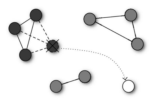
The remaining particles, which were removed from the overcrowded clusters and reinitialized, are used to explore the search space for possible new interesting areas. In the first implementation of the algorithm, these unniched particles had no connections, thus they performed the kind of nondeterministic hill-climbing associated with the cognition-only model [5]. However, the first experiments showed that the poor capabilities of this model hindered the search for new solutions, leading to a less-than-optimal performance on complex functions.
Thus, we modified the kPSO algorithm so that the unniched particles are organized in a von Neumann lattice neighborhood (see Figure 4). In this way, when particles are reinitialized, they start performing a more efficient search for new solutions, which allows the algorithm to identify all the multiple optima.
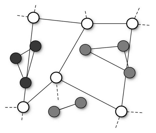
Once the neighborhood structure has been set both for the niched and the unniched particles, the algorithm performs a fixed number c of steps of the constriction-factor PSO. In this phase there are only two aspects in which kPSO differs from the standard algorithm.
- (i)
The particles assigned to a niche Cj will have their velocities clamped to Vmax = 2σj (see (8)), which is proportional to the width of the cluster.
- (ii)
The unniched particles will behave as in a constriction-factor PSO with the von Neumann lattice topology.
After c steps, the clustering and cutting procedures are repeated. The pseudocode for kPSO is reported in Algorithm 2.
-
Algorithm 2: kPSO algorithm
pseudocode.
-
procedure kPSO
-
Initialize particles with random positions and velocities.
-
Set particles′ pbests to their current positions.
-
Calculate particles′ fitness.
-
for step t = 0 → T − 1do
-
ift mod c = 0then Every c steps.
-
Execute the procedure Identify Niches.
-
end if
-
Update particles′ velocities. Perform the standard PSO step.
-
Update particles′ positions.
-
Recalculate particles′ fitness.
-
Update particles′ and neighborhood best positions.
-
end for
-
end procedure
The application of the kPSO algorithm requires to set a few additional parameters with respect to the standard PSO. We already discussed the first one, c, the number of PSO steps between two clustering applications.
The second parameter for the k-means algorithm is k, the number of clusters, which is also the most problematic. In fact, the value for k that leads to the best performance of the algorithm is strongly dependent on the number m of optima of the function under consideration. When the latter is known, k can be set to a value which is slightly larger than it. In this way, the algorithm will maintain a sufficient number of clusters to be able to identify all the optima, while possibly forming spurious clusters, that is, clusters not corresponding to any optima.
Regarding those parameters which are in common with the standard constriction-factor PSO, we used the common values of pincr = gincr = 2.05 and χ≃0.730.
4.3. Estimating the Number of Clusters
One of the major issues with our approach in kPSO is the fact that one needs to specify the number of clusters k, which is strongly related to the number of optima of the function under consideration. Unfortunately, often the number of optima of a function cannot be estimated a priori; rather, it would be desirable that it could be discovered by the optimization algorithm itself.
The need to know the number of clusters is inherited by kPSO from the specific clustering algorithm we chose, k-means, although it is a problem which is common to a wide class of clustering algorithms. Significant research has focused on the problem of estimating k, using very different approaches [30]. Here we will discuss an approach which leads to the estimation of k by the optimization of a criterion function in a probabilistic mixture-model framework.
Next, ρ(x∣Cj,θj) is the conditional probability distribution associated with the same cluster (component density). Finally, θ = (θ1, … ,θk) is the vector of the parameters of the distributions for all clusters.
It has been proven [29] that the k-means algorithm implicitly performs a maximization of the likelihood under the assumption that the component densities are spherical Gaussian distributions.
Extending on these considerations, finding the number of clusters k is equivalent to fitting the model with the observed data and optimizing some criterion. This can be done by applying the k-means algorithm with k varying in a range of possible values and then choosing the best clustering.
However, the problem arises of choosing a valid criterion to select the best clustering. Here the maximum likelihood is not helping, since it invariably leads to the choice of the highest k. Thus, a large number of alternative criteria have been proposed, which combine concepts from information theory. The most typical examples include the Akaike′s information criterion (AIC) [32, 33] and the Bayesian information criterion (BIC) [34, 35].
4.3.1. The Bayesian Information Criterion
In the improved version of the kPSO algorithm, at each clustering application, k-means is thus repeated with varying values for k (usually in the range from 2 to N/2), then the clustering with the highest BIC is chosen. In this way, there is no need to set a value for k at the beginning of the run. Rather, it can vary across the execution of the algorithm, as the particles in the swarm slowly discover new promising areas and organize in new niches.
5. Experiments
In [28], we presented a first version of the kPSO algorithm without the automatic selection of the number of clusters and evaluated its performance in comparison to those of NichePSO [15] and parallel vector-based PSO [20]. Results showed how kPSO could achieve similar or better results, requiring quite low computational resources.
Thus, in this study we chose to compare the enhanced version of kPSO with automatic selection of the number of clusters (see Section 4.3.1) with other two niching algorithms, the SPSO [21] and ANPSO [25] algorithms, which probably represent the state-of-the-art of niching algorithms for the particle swarm. The study was conducted on the same set of benchmark functions used in [25] and reported in Table 1.
| Function | Equation | Domain |
|---|---|---|
| Branin RCOS | ||
| Six-Hump camel back | ||
| Deb′s 1st function | M3(x) = sin 6(5πx) | 0 ≤ x ≤ 1 |
| Himmelblau | −6 ≤ x, y ≤ 6 | |
| Shubert 2D | −10 ≤ x, y ≤ 10 |
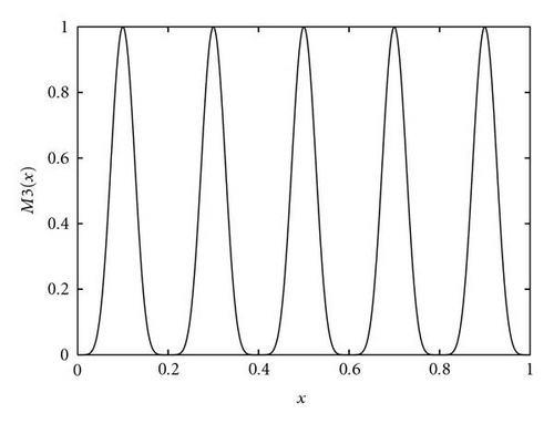
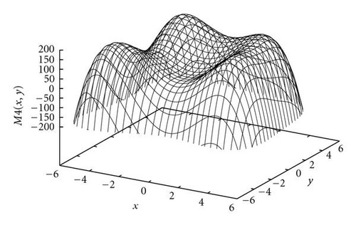
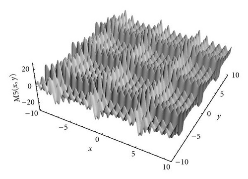
The first function in the study was the Branin RCOS function, a two-dimensional function with 3 global optima in the region we considered (see Figure 5). The second function was the six-hump camel back (Figure 6), with only 2 global optima, but several deceptive local ones. The third function, the Deb′s 1st function, was a one-dimensional function with 5 equally spaced global optima (see Figure 7). The fourth one was the Himmelblau function (Figure 8), again two-dimensional, with 4 global optima. Finally, the 5th and last function of the study was the Shubert 2D function, with 18 global optima grouped in 9 clusters and surrounded by a very high number of local optima (Figure 9).
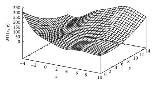

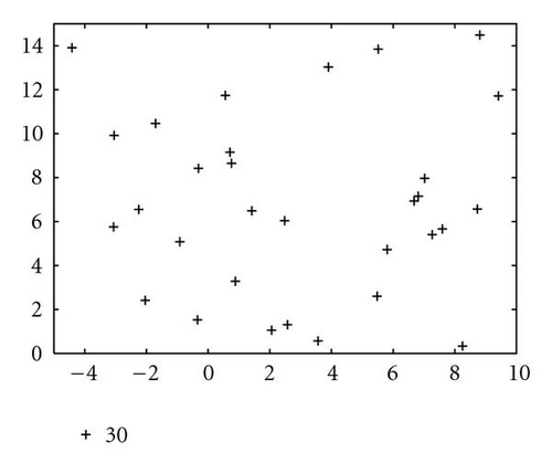
In order to show how the improved version of our algorithm can effectively identify niches surrounding the optima of a function, we report in Figure 10 several significant steps of kPSO running on the Branin RCOS function M1. In the snapshots we plotted, it is shown how at the beginning of the run the particles of the swarm are randomly distributed on the search space. Then, during the first steps of the particle swarm simulation, they naturally start to split in different groups, roughly adapting to the fitness landscape.
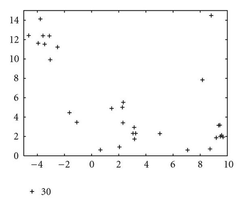
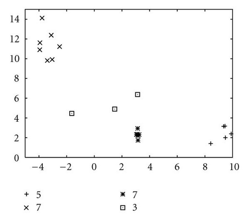
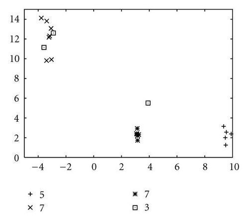
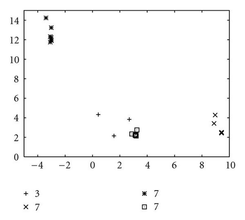
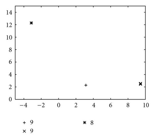
When the first clustering application occurs (see Figure 10(c)), it identifies 4 niches, 3 of which actually correspond to the global optima, while the other is a spurious one. In the particular case that is shown here, the algorithm will eventually converge to exactly 3 clusters, as it is shown in Figure 10(f), at the 62nd simulation step. However, such convergence is not the final goal of kPSO: as long as a sufficient number of clusters has formed to cover all the optima, the presence of spurious clusters is really of no harm to the optimization algorithms. Besides, in early phases of the optimization, the presence of additional clusters can be helpful in locating new interesting regions of the search space.
In Table 2 we report the results obtained on the five benchmark functions with kPSO, SPSO, and ANPSO. The experiments were carried out so that for each function the optimization algorithm was executed with two different populations sizes. Each execution was repeated 50 times, setting the threshold for the maximum number of iteration to 2000 simulation steps.
| Function | Particles | SPSO | ANPSO | kPSO |
|---|---|---|---|---|
| M1 | 30 | 3169 ± 692 | 5220 ± 3323 | 2084 ± 440 |
| 60 | 6226 ± 1707 | 6927 ± 2034 | 3688 ± 717 | |
| M2 | 30 | 2872 ± 827 | 2798 ± 857 | 1124 ± 216 |
| 60 | 5820 ± 1469 | 4569 ± 1316 | 2127 ± 341 | |
| M3 | 30 | 2007 ± 703 | 6124 ± 2465 | 1207 ± 688 |
| 60 | 4848 ± 2092 | 8665 ± 2974 | 1654 ± 705 | |
| M4 | 30 | 4096 ± 731 | 16308 ± 13157 | 2259 ± 539 |
| 60 | 7590 ± 2018 | 17168 ± 12006 | 3713 ± 570 | |
| M5 | 300 | 166050 ± 42214 | 82248 ± 10605 | 81194 ± 45646 |
| 500 | 219420 ± 80179 | 114580 ± 18392 | 117503 ± 77451 |
In all the experiments, the goal of the optimization algorithm was to locate all the global optima with an accuracy of ϵ = 0.00001 and to maintain all of them for at least 10 simulation steps. Since all the algorithms could actually fulfill the goal within the maximum number of 2000 iterations, we only report in Table 2 their performance in term of the number of function evaluations they required.
The first four functions in the benchmark, M1, … ,M4, proved to be quite easy to optimize. A population size of just 30 particles was more than sufficient to identify all the global optima with a quite low number of function evaluations. In Table 2, we report also the results with a population of 60 particles in order to compare them to those in [25]. kPSO proved to have a clear advantage on all of these functions with respect to SPSO and ANPSO.
In the experiments with functions M1 to M4 we used a value of c = 10 for the number of steps between two clustering applications. With higher values, the performance of the algorithm did not vary significantly, meaning that it was a sufficient number of steps for the particles to adjust to the changed social structure after a clustering application.
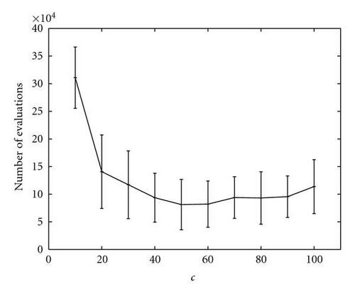
A special analysis was conducted regarding the optimization of function M5, which was the most complex function of the set, in particular because it presented many local optima surrounding the global ones. As shown in Figure 11, even if kPSO was able to find all the optima in all the runs, the number of evaluations required changed greatly depending on the value of c. A small value for c would hamper the tendency of the particles to follow the standard PSO dynamics, since they would be rearranged in different clusters too often. A too high value would instead freeze the swarm on fixed clusters for a long time, resulting in worse performance, since a high number of function evaluations would be wasted. We found that a good value was c = 50, so we used it for the other experiments (Table 2 and Figure 12).
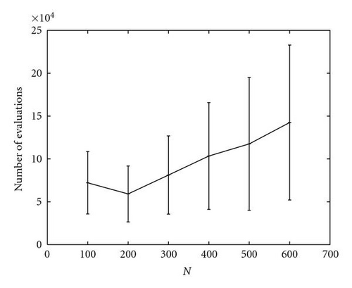
The higher degree of complexity of function M5 also led to the use of a much larger population. In the experiments reported in Table 2, we employed the two population sizes of 300 and 500 in order to compare the results to those of ANPSO and SPSO as reported in [25]. The performance of kPSO appears to be quite better than those of SPSO and comparable to those of ANPSO, although they exhibits a larger variance over the 50 runs. However, kPSO successfully located all the optima in M5 also with smaller population sizes, as plotted in Figure 12, requiring rather fewer function evaluations than the other algorithms. In particular, with a population of only 200 particles, kPSO was able to locate all the global optima performing just 59165 ± 32646 function evaluations.
The set of experiments was intended to test the performance of the improved version of kPSO and to compare it with two of the best existing niching PSO algorithms, SPSO and ANPSO. The results we obtained were quite good: the kPSO algorithm, with the new mechanism to adaptively determine the number of clusters, outperformed the other algorithms by a good margin on most of the test functions.
The situation was rather more elaborated regarding the most complex function of the group, the Shubert 2D function. In this case, kPSO still showed very good results on average, but also a very large variance. Moreover it needed an adjustment of the newly introduced parameter, the number of simulation steps between two clustering applications. In fact, while for the simple functions this number was kept constant at a quite low value, the application to the Shubert function required a much higher value, in a way that is consistent with what we found out in earlier experiments on the influence of c.
5.1. Computational Cost
Another important aspect to consider in the evaluation of the different approaches to niching is the computational cost of the niching procedure itself. In general, when considering the efficiency of an optimization algorithm, the most significant measure is the one we used in our last experiments, that is the number of function evaluations the algorithm requires to reach the predefined goal. In fact, calculating the function value is usually the single operation with the highest computational cost in a real-world problem.
However, in certain cases, the computational overhead added by other operations required by the optimization algorithm should be taken into account. In the comparison we are discussing, all the algorithms implement a version of the particle swarm approach, thus they share roughly the same (quite low) computational costs related to the simulation of particles′ dynamics. In this regard, the only aspect in which they differ is the specific niching procedure they use. The computational cost of these procedures can be evaluated in terms of the number of distance calculations. For the SPSO algorithm, this leads to a computational cost at each iteration that is O(N · k), where N is the swarm size and k the number of seeds or niches. The ANPSO algorithm, instead, implements a more complex procedure, which has a cost of O(N2).
Our approach basically inherits the computational complexity of the k-means algorithm, that is O(N · k · rk). But considering that the improved version actually repeats the k-means application in order to determine the best number of clusters, the final computational cost is in the order of O(N2 · rk). It should be noted, however, that kPSO, unlike the other algorithms, only executes the niching procedure every c simulation steps, thus reducing its computational overhead by the same factor. Considering the order of magnitude of the parameters rk and c we used in all the experiments, the average cost per iteration is O(N2 · rk/c)≃O(N2), therefore in the same order as ANPSO. A summary of the computational overhead of the various niching procedure, averaged per single iteration, is given in Table 3.
| Algorithm | Cost |
|---|---|
| SPSO | O(N · k) |
| ANPSO | O(N2) |
| kPSO | O(N2 · rk/c)≃O(N2) |
While in this analysis it emerges that the SPSO algorithm is the one which adds the lowest computational overhead to identify niches, compared to ANPSO and kPSO, whether this is really important or not depends mainly on two factors.
- (i)
In many real-world optimization problems, the most relevant component of the computational cost is the number of function evaluations. Thus, an algorithm with a highest overhead in term of distance calculations, but which requires significantly less evaluations, is surely to be preferred.
- (ii)
Fine-tuning the parameters adds another computational cost. This is just one of the main issues Bird and Li tried to assess with the introduction of ANPSO over SPSO. The latter, in fact, requires the specification of a fixed niche radius, thus it realistically needs to be executed multiple times to find the best value, while ANPSO can adaptively determine it during a single run. In this regard, kPSO is more similar to ANPSO, as it can adaptively determine k, the most problem-dependent parameter. However, it still needs a value for c to be chosen, which can significantly influence its efficiency, but does not really hinder its ability to locate all the optima.
6. Conclusions
In this paper, we introduced a new approach to niching in particle swarm optimization based on clustering. Then we described kPSO, our implementation which uses the k-means clustering algorithm to identify niches and the Bayesian information criterion to determine the number of clusters. The resulting algorithm maintains essentially the same structure as the standard PSO. In fact the niching effect is obtained just by influencing the neighborhood structure of the swarm, while the dynamics of the single particles remain unchanged. Thus, each subswarm created by the clustering process performs a local search with the same efficiency as the standard PSO.
The kPSO algorithm was competitive with other niching algorithms for the particle swarm. In particular, it markedly outperformed one of the best existing algorithms, SPSO, in term of the number of function evaluations needed to discover all the optima of the test functions. Even though the computational cost of the clustering procedure in kPSO is higher than that of SPSO, we thought that it is balanced by the improved ability to adapt with far less manual tuning to different function landscapes, and by the sensible gain in performance. In this respect, the advantages of kPSO are rather similar to those of ANPSO, another interesting algorithm which adaptively determines the main niching parameters. The two algorithms, in fact, introduce a comparable computational overhead with the procedure to identify niches. kPSO, however, showed higher or comparable performance in all the tests we conducted.
Research on the clustering approach will continue in several directions. To begin with, the kPSO algorithm will be put to test with higher-dimensionality benchmark functions together with real-world problems in order to better assess its capabilities. Another interesting research line involves the development of a more flexible version of kPSO, which will avoid the need to set c, the number of steps between clusterings. This could be accomplished for example by developing an algorithm which could estimate when a new clustering application is needed, rather than performing it at fixed intervals. Further research will also be devoted to investigate the employment of different clustering algorithms rather than the k-means.


