Constructing Reservoir Flow Simulator Proxies Using Genetic Programming for History Matching and Production Forecast Uncertainty Analysis
Abstract
Reservoir modeling is a critical step in the planning and development of oil fields. Before a reservoir model can be accepted for forecasting future production, the model has to be updated with historical production data. This process is called history matching. History matching requires computer flow simulation, which is very time-consuming. As a result, only a small number of simulation runs are conducted and the history-matching results are normally unsatisfactory. This is particularly evident when the reservoir has a long production history and the quality of production data is poor. The inadequacy of the history-matching results frequently leads to high uncertainty of production forecasting. To enhance the quality of the history-matching results and improve the confidence of production forecasts, we introduce a methodology using genetic programming (GP) to construct proxies for reservoir simulators. Acting as surrogates for the computer simulators, the “cheap” GP proxies can evaluate a large number (millions) of reservoir models within a very short time frame. With such a large sampling size, the reservoir history-matching results are more informative and the production forecasts are more reliable than those based on a small number of simulation models. We have developed a workflow which incorporates the two GP proxies into the history matching and production forecast process. Additionally, we conducted a case study to demonstrate the effectiveness of this approach. The study has revealed useful reservoir information and delivered more reliable production forecasts. All of these were accomplished without introducing new computer simulation runs.
1. Introduction
Petroleum reservoirs are normally large and geologically complex. In order to make management decisions that maximize oil recovery, reservoir models are constructed with as many details as possible. Two types of data that are commonly used in reservoir modeling are geological data and production data. Geological data, such as seismic and wire-line logs, describe earth properties, for example, porosity, of the reservoir. In contrast, production data, such as water saturation and pressure information, relate to the fluid flow dynamics of the reservoir. Both data types are required to be honored so that the resulting models are as close to reality as possible. Based on these models, managers make business decisions that attempt to minimize risk and maximize profits.
The integration of production data into a reservoir model is usually accomplished through computer simulation. Normally, multiple simulations are conducted to identify reservoir models that generate fluid dynamics matching the historical production data. This process is called history matching.
History matching is a challenging task for the following reasons.
- (i)
Computer simulation is very time consuming. On average, each run takes 2 to 10 hours to complete.
- (ii)
This is an inverse problem where more than one reservoir model can produce flow outputs that give acceptable match to the production data.
As a result, only a small number of computer simulation runs are conducted and the history matching results are associated with uncertainty. This uncertainty also translates into the uncertainty of future production forecasts. In order to optimize reservoir planning and development decisions, it is highly desirable to improve the quality of the historical matching results. The subject of uncertainty in reservoir modeling and production forecast has been studied intensively for the past few years (see Section 2).
Previously, we have introduced a methodology using genetic programming (GP) [1, 2] to construct a reservoir flow simulator proxy to enhance the history matching process [3]. Unlike the full reservoir simulator, which gives the flow of fluids of a reservoir, this proxy only labels a reservoir model as “good” or “bad”, based on whether or not its flow outputs match well with the production data. In other words, this proxy acts as a classifier to separate “good” models from “bad” models in the reservoir descriptor parameter space. Using this “cheap” GP proxy as a surrogate of the full-simulator, we can examine a large number of reservoir models in the parameter space in a short period of time. Collectively, the identified good-matching reservoir models provide us with comprehensive information about the reservoir with a high degree of certainty.
In this contribution, we applied the developed method to a West African oil field which has a significant production history and noisy production data. Additionally, we carried out production forecast using the history matching results. Production forecast also required computer simulation. Since the number of good models identified by the history-matching proxy was large, it was not practical to make all these computer simulation runs. Similar to the way the history-matching proxy was constructed, a second reservoir proxy was constructed for production forecast. This proxy was then applied to the good reservoir models to forecast future production. Since the forecasting was based on a large number of reservoir models, it was closer to reality than the forecasts derived from a small number of computer simulation runs.
Overall, the project has successfully achieved the goal of enhancing the quality of the history-matching models and improving the confidence of production forecast, without introducing new reservoir simulation runs. We believe that the proposed methodology is a cost-effective way to achieve better reservoir planning and development decisions.
The rest of the paper is organized as follows. Section 2 explains the process of reservoir history matching and production forecast. The developed methodology and its associated workflow are then presented in Section 3. In Section 4, we describe the case study of a West African oil field. Details of data analysis and outliers detection are reported in Section 5. Following the proposed workflow step by step, we present our history matching study in Section 6 and give the production forecast analysis in Section 7. We discuss computer execution time in Section 8. Finally, Section 9 concludes the paper with suggestions of future work.
2. History Matching and Production Forecast
When an oil field is first discovered, a reservoir model is constructed utilizing geological data. Geological data can include porosity and permeability of the reservoir rocks, the thickness of the geological zones, the location and characteristics of geological faults, and relative permeability and capillary pressure functions. Building reservoir models using geological data is a forward modeling task and can be accomplished using statistical techniques [4] or soft computing methods [5].
Once the field enters into the production stage, many changes take place in the reservoir. For example, the extraction of oil/gas/water from the field causes the fluid pressures of the field to change. In order to obtain the most current state of a reservoir, these changes need to be reflected in the model. History matching is the process of updating reservoir descriptor parameters to reflect such changes, based on production data collected from the field. Using the updated models, petroleum engineers can make more accurate production forecasts. The results of history matching and subsequent production forecasting strongly impact reservoir management decisions.
History matching is an inverse problem. In this problem, a reservoir model is a black box with unknown parameters values (see Figure 1). Given the water/oil rates and other production information collected from the field, the task is to identify these unknown parameter values such that the reservoir model gives flow outputs matching production data. Since inverse problems, typically, have no unique solutions, that is, more than one combination of reservoir parameter values give the same flow outputs, we need to obtain a large number of well-matched reservoir models in order to achieve high confidence in the history-matching results.
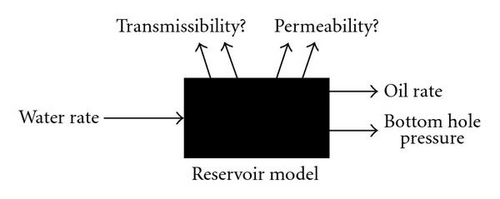
Figure 2 depicts the work flow of history matching and production forecast process. Initially, a base geological model is provided. Next, parameters which are believed to have an impact on the reservoir fluid flow are selected. Based on their knowledge about the field, geologists and petroleum engineers determine the possible value ranges of these parameters and use these values to conduct computer simulation runs.
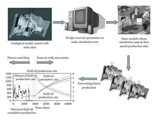
A computer reservoir simulator is a program which consists of mathematical equations that describe fluid dynamics of a reservoir under different conditions. The simulator takes a set of reservoir parameter values as inputs and returns a set of fluid flow information as outputs. The outputs are usually a time-series over a specified period of time. That time-series is then compared with the historical production data to evaluate their match. If the match is not satisfactory, experts would modify the parameters values and make a new simulation run. This process continues until a satisfactory match between simulation flow outputs and the production data is reached.
This manual process of history matching is subjective and labor-intensive, because the reservoir parameters are adjusted one at a time to refine the computer simulations. Meanwhile, the quality of the matching results largely depends on the experience of the geoscientists involved in the study. Consequently, the reliability of the forecasting is often very short lived, and the business decisions made based on those models have a large degree of uncertainty.
To improve the quality of history matching results, several approaches have been proposed to assist the process. For example, gradient-based algorithms have been used to select sampling points sequentially for further computer simulations [7]. Although this approach can quickly find models that match production data reasonably well, it may cause the search to become trapped in a local optimum and prevent models with better matches being discovered. Another shortcoming is that the method generates a single solution, despite the fact that multiple models can match the production data equally well. To overcome these issues, genetic algorithms have been proposed to replace gradient-based algorithms [8, 9]. Although the results are significantly better, the computation time is not practical for large reservoir fields.
There are also several works that construct a response surface that reproduces the approximate reservoir simulation outcomes. The response surface is then used as a surrogate or proxy for the costly full simulator [10]. In this way, a large number of reservoir models can be sampled within a short period of time.
Response surfaces are normally polynomial functions. Recently, kriging interpolation and neural networks have also been used as alternative methods [11, 12]. The response surface approach is usually carried out in conjunction with experimental design, which selects sample points for computer simulation runs [13]. Ideally, these limited number of simulation runs would obtain the most information about the reservoir. Using these simulation data to construct a response surface estimator, it is hoped that the estimator will generate outcomes that are close to the outcomes of the full simulator. This combination of response surface estimation and experimental design is shown to give good results when the reservoir models are simple and the amount of production data is small, that is, the oil field is relatively young [6]. However, when the field has a complex geologic deposition or has been in production for many years, this approach is less likely to produce a quality proxy [14]. Consequently, the generated reservoir models contain a large degree of uncertainty.
3. A Genetic Programming Solution
To improve the quality of the reservoir models generated from history matching, a dense distribution of reservoir models needs to be sampled. Additionally, there needs to be a method for identifying which of those models provide a good match to the production data history of the reservoir. With that information, only “good” models will be used in the analysis for estimating future production and this will result in greater confident in the forecasting results.
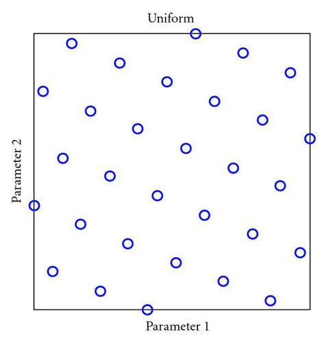
To achieve that goal, we have adopted uniform design to conduct computer simulation runs and applied genetic programming for proxy construction. Uniform design, developed by Fang [15], generates a sampling distribution that covers the entire parameter space for a predetermined number of runs. It ensures that no large regions of the parameter space are left undersampled. Such coverage is important to obtain simulation data for the construction of a robust proxy that is able to interpolate all intermediate points in the parameter space.
In terms of implementation, we first decide the number of simulation runs based on the complexity of the reservoir. We then apply the Hammersley algorithm [16] to distribute parameter values of these runs to maximize the coverage. Figure 3 shows a case where the sampling points were distributed to cover a 2-parameter space. The algorithm works similarly to parameter spaces with a larger dimension. This sampling strategy gives better coverage than that by the random Monte Carlo method.
Using the simulation results, we then apply GP symbolic regression to construct a proxy. Unlike other research works where the proxy is constructed to give the same type of output as the full simulator [12], this GP proxy only labels a reservoir model as a good match or bad match to the production data, according to the criterion decided by field engineers. In other words, it functions as a classifier to separate “good” models from “bad” ones in the parameter space. The actual amount of fluid produced by the sampled reservoir models is not estimated. This is a different kind of learning problems and it will be shown that GP is able to learn the task very well.
After the GP classifier is constructed, it is then used to sample a dense distribution of reservoir models in the parameter space (millions of reservoir models). Those that are labeled as “good” are then studied and analyzed to identify their associated characteristics. Additionally, we will use these “good” models to forecast future production. Since the forecast is based on a large number of good models, the results are considered more accurate and closer to reality than those based on a limited number of simulation runs.
With the inclusion of these extra steps, the workflow of reservoir history matching and production forecasting is shown as in Figure 4. Initially, reservoir parameters and their value ranges are decided by experts (step 1). Next, the number of simulation runs and the associated parameters values are determined according to uniform design (step 2). Based on this setup, computer simulations are conducted (step 3). After that, the objective function and the matching threshold (the acceptable mismatch between simulation results and production data) are defined (step 4). Those reservoir models that pass the threshold are labeled as “good” while the others are labeled as “bad” (step 5). These simulation results are then used by GP symbolic regression to construct a proxy that separates good models from bad models (step 6). With this GP classifier as the simulator proxy, we can then sample a dense distribution of the parameter space (step 7). The models that are identified by the classifier as “good” are selected for forecasting future production (step 8).
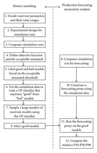
Reservoir production forecast also requires computer simulation. Since the number of “good” models identified by the GP-proxy is normally large, it is not practical to make all these runs. Similar to the way the simulator proxy is constructed for history matching, a second GP proxy is generated for production forecast. However, unlike the history-matching proxy, which is a classifier, forecasting proxy is a regression which outputs a production forecast value. As shown on the right-hand side of Figure 4, the simulation results based on uniform sampling (step 9) will be used to construct a GP forecasting proxy (step 10). This proxy is then applied to all “good” models identified by the history-matching proxy (step 11). Based on the forecasting results, uncertainty statistics such as P10, P50, and P90 are estimated (step 12).
4. A Case Study
The case study is conducted on a large oil field in West Africa. It has over one billion barrels of original oil in place and has been in production for more than 30 years. Due to the long production history, the data collected from the field were not consistent and the quality was not reliable. Although we do not know for sure what causes the production measurements to be inaccurate, we could speculate on newer technology but more likely it is just poor measurement taking from time to time. We will address this data quality issue in Section 5.
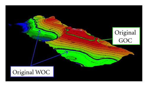
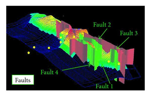
This field is overlain by a significant gas cap. Figure 5 shows the oil field and the gas oil contact (GOC) surface that separates the gas cap from the underneath oil. Similarly, there is a water oil contact (WOC) surface that separates oil from the water below. The space between GOC and WOC surfaces is the oil column to be recovered. The field also has 4 geological faults, illustrated in Figure 6, which affect the oil flow patterns. Those faults have to be considered in the computer flow simulation.
As a mature field with most of its oil recovered, the reservoir now has pore space which can be used for storage. One proposed plan is to store the gas produced as a side product from the neighboring oil fields. In this particular case, the gas produced has no economical value and reinjecting it back into the field was one environmental-friendly method of storing the gas.
In order to evaluate the feasibility of the plan, the cumulative volume of gas that can be injected (stored) in year 2031 needed to be evaluated. This evaluation would assist managers in making decisions such as how much gas to transport from the neighboring oil fields and the frequency of the transportation.
The cumulative volume of the gas that can be injected is essentially the cumulative volume of the oil that will be produced from the field, since this is the amount of space that will become available for gas storage. To answer that question, a production forecasting study of this field in the year 2031 has to be conducted.
Prior to carrying out production forecast, the reservoir model has to be updated through the history matching process. The first step, as described in Figure 4, is deciding reservoir parameters and their value ranges for flow simulation. After consulting with field engineers, 10 parameters were selected (see Table 1). All parameters are unit-less except WOC and GOC, whose unit is feet. Critical gas saturation (SGC) is the gas saturation values for each phase (water and oil), which has a value between 0 to 1. Skin at new gas injection (SKIN) is the rock formation damage caused by the drilling of new gas injector wells. It has values between 0 and 30. The rest 6 parameters are multipliers and are in log 10 scale.
| Parameters | Min | Max |
|---|---|---|
| Water oil contact (WOC) | 7289 feet | 7389 feet |
| Gas oil contact (GOC) | 6522 feet | 6622 feet |
| Fault transmissibility multiplier (TRANS) | 0 | 1 |
| Global Kh multiplier (XYPERM) | 1 | 20 |
| Global Kv multiplier (ZPERM) | 0.1 | 20 |
| Fairway Y-Perm multiplier (YPERM) | 0.75 | 4 |
| Fairway Kv multipilier2 (ZPERM2) | 0.75 | 4 |
| Critical gas saturation (SGC) | 0.02 | 0.04 |
| Vertical communication multiplier (ZTRANS) | 0 | 5 |
| Skin at new gas injection (SKIN) | 0 | 30 |
During computer simulation, the 10 parameter values are used to define the reservoir properties in each grid of the 3D model in two different ways. The values of the 4 regular parameters are used to replace the default values in the original 3D model while the 6 multipliers are applied to the default values in the original model. Computer simulations are then performed on the updated reservoir models to generate flow outputs.
The parameters selected for computer simulation contain not only the ones that affect the history like fluid contacts (WOC and GOC), fault transmissibility (TRANS), permeability (YPERM), and vertical communication in different area of the reservoir (ZTRANS), but also parameters associated with future installation of new gas injection wells, such as skin effect (SKIN). When a well is drilled, the rock formation is typically damaged around the well. If the damage is small, the “skin effect” value is close to 0. If the formation around the well is severely impacted by the drilling, the “skin effect” value can be as high as 30. “Skin effect” acts as an additional resistance to flow. By including parameters associated with future production, each computation simulation can run beyond history matching and continue for production forecast to the year 2031. With these setup, each computer simulation produces the flow outputs time-series data for both history matching and for production forecasting. In other words, step 3 and 9 are carried out simultaneously.
Based on uniform design, parameter values are selected to conduct 600 computer simulation runs (step 2 and 3). Each computer simulation takes about one hour to complete using a single CPU machine. For a quick turnover of the results, we used computer clusters to process dozens of simulations at the same time. We have several computer clusters in the company, each has typically hundreds of nodes (128 for instance) but only 10–20 nodes are available per user at a given time. In this case, the total running time for the simulation was in the order of days.
Among the 600 runs, 593 were successful in that the runs continued until year 2031. The other 7 runs failed for various reasons, such as power failures, and terminated before the runs reached year 2031.
During the computer simulation, various flow data were generated. Among them, only field water production rate (FWPR) and field gas production rate (FGPR), from year 1973 to 2004, were used for history matching. The other flow data were ignored because we do not trust the quality of their corresponding production data collected from the field.
FWPR and FGPR collected from the field were compared with the simulation outputs from each run. The “error” E, defined as the mismatch between the two, is the sum-squared error calculated as follows:
Here, “obs” indicates production data while “sim” indicates computer simulation outputs. The largest E that can be accepted as good match is 1.2 (step 4 in Figure 4). Additionally, if a model has E smaller than 1.2 but has any of its FWPR or FGPR simulation outputs match badly to the corresponding production data (difference is greater than 1), the production data was deemed not to be reliable and the entire simulation record is disregarded. Based on this criterion, 12 data points were removed. For the remaining 581 simulation data, 63 were labeled as “good” models while 518 were labeled as “bad” models (step 5 in Figure 4).
5. Data Analysis and Outliers Detection
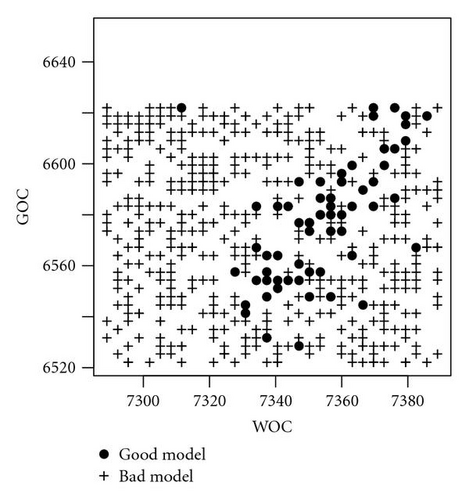
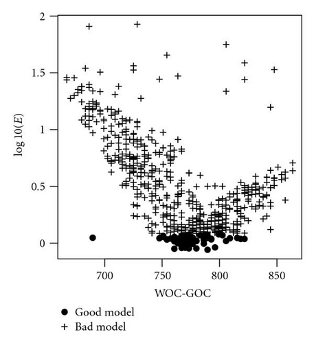
To solve the history-matching problem, we need to find parameter values that produce fluid flow matching the production data. Previously, a history-matching study on this field has reported that oil column (WOC-GOC) has a strong impact on the reservoir flow outputs, hence it is important to the matching of production data [11]. As shown in Figure 7, among the 581 simulation data, all 63 good models have their WOC and GOC correlated: when the WOC is low, its GOC is also low, thus preserving the oil column. This suggests that only a particular range of oil column heights might be able to satisfy history matching. To investigate if this is true, we added the oil column variable (WOC-GOC) to the parameter set. This new variable might help reducing the complexity of the proxy construction (see Figure 8).
Before proceeding to step 6 of GP proxy constructing, we decided to perform an outliers study on the 581 simulation/production data due to the poor quality of the production data. This is a common practice in data modeling when the data set is noisy or unreliable.
The following rationale was used to detect inconsistent production data. Reservoir models parameter values and the produced flow outputs generally have a consistent pattern. The computer simulator is an implementation of that pattern to map reservoir parameters values to flow outputs. Similarly, there is a consistent pattern between reservoir parameter values and the mismatch (E) of simulator outputs and production data. If the mismatching E of a data point was outside the pattern, it indicated that the production data had a different quality from the others and should not be trusted. Based on this concept, we used GP symbolic regression to identify the function that describes the pattern between reservoir parameter values and E. The GP system and the experimental setup are given in the following subsection.
5.1. Experimental Setup
This case study used a commercial GP package [17]. In this system, some GP parameters were not fixed but were selected by the software for each run. These GP parameters included population size, maximum program size, and crossover and mutation rates. In the first run, one set of values for these GP parameters was generated. When the run did not produce an improved solution for a certain number of generations, the run was terminated and a new set of GP parameter values was selected by the system to start a new run. The system maintained the best 50 solutions found throughout the multiple runs. When the GP system was terminated, the best solution among the pool of 50 solutions was the final solution. In this work, the GP system continued for 120 runs and then was manually terminated.
In addition to the parameters whose values were system generated, there were other GP parameters whose values needed to be specified by the users. Table 2 provides the values of those GP parameters for the outliers study. The terminal set consists of the 11 reservoir parameters, each of which could be used to build the leaf node in the GP regression trees. The target is E, which was compared to the regression output R for fitness evaluation. The fitness of an evolved regression was the mean squared error (MSE) of the 581 data points. A tournament selection with size 4 is used to select winners. In each tournament, 4 individuals were randomly selected to make 2 pairs. The winners of each pair became parents to generate 2 offspring.
| Objective | Evolve a regression to identify outliers in production data. |
|---|---|
| Functions | Addition, subtraction, multiplication, division, abs |
| Terminals | The 10 reservoir parameters listed in Table 1 & oil column |
| Fitness | MSE: , R is regression output. |
| Selection | Tournament (4 candidates/2 winners) |
5.2. Results
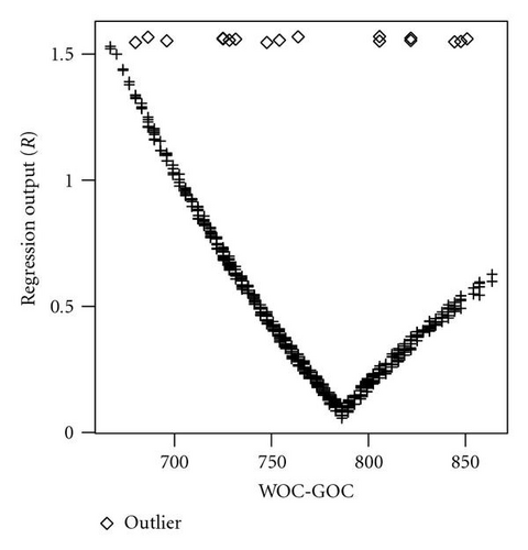
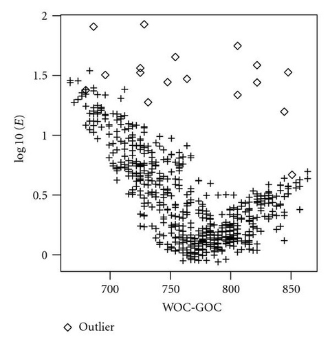
At the end of 120 runs, the best GP regression contained 4 parameters: WOC-GOC, TRANS, YPERM, and SGC. Among them, WOC-GOC was ranked as having the most impact on the match of production data. Figure 9 shows the relationship between WOC-GOC and the regression outputs R. It is evident that 17 of the data points did not fit into the regression pattern. These 17 data points also had similar outliers behavior with regard to E (see Figure 10). These are clear evidences that the 17 production data points were unreliable and were removed from the data set.
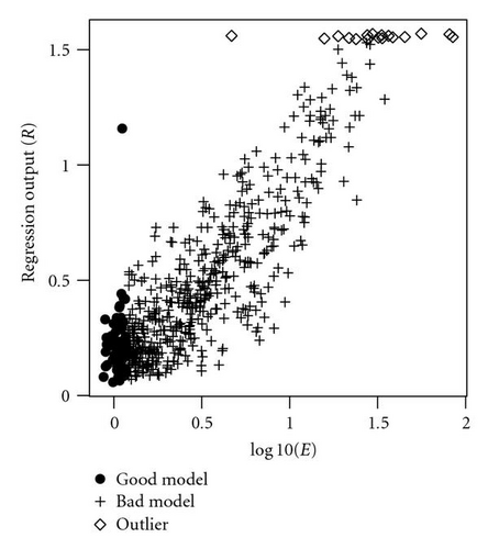
After the outliers were removed, the final data set to construct the simulator proxies consisted of 564 data points; 63 of them were good models while 501 were bad models as illustrated in Figure 11. The outliers study was then completed.
6. History-Matching Study
The next step, step 6, in the history-matching study was to construct the reservoir simulator proxy which classified a reservoir model is “good” or “bad” based on the given reservoir parameter values. For this step, the final set of 564 data points were used to construct this GP classifier. Each data point contained 4 input variables (WOC-GOC, TRANS, YPERM, and SGC), which were selected by the GP regression outliers study, and one output, E.
With the number of “bad” models 8 times larger than the number of “good” models, this data set was very unbalanced. To avoid GP training process generating classifiers that biased “bad” models, the good model data were replicated 5 times to balance the data set. This ad hoc approach has allowed GP to produce classifiers with better accuracy and robustness than that generated based on the data without replication. However, there are other more systematic approaches to address the data imbalance problem. Some examples are oversampling of small class, undersampling of large class, and modifying the relative cost associated to misclassification so that it compensates for the imbalance ratio of the two classes [18, 19]. We will investigate these methods and compare their effectiveness on this data set in our future study.
Normally, we split the data set into training, validation and testing to avoid overfitting. However, because the number of good models was very small and splitting them further would have made it impossible for GP to train a proxy that represented the full simulator capability, we used the entire set as training data to construct the proxy.
6.1. Experimental Setup
The GP parameter setup for this experiment was different from the setup for the outliers study. In particular, the fitness function was not MSE. Instead, it was based on hit rate: the percentage of the training data that were correctly classified by the regression. Table 3 includes the GP system parameters values for symbolic regression to evolve the history matching proxy.
| Objective | Evolve a simulator proxy classifier for history matching. |
|---|---|
| Functions | Addition, subtraction, multiplication, division, abs |
| Terminals | WOC-GOC, TRANS, YPERM, SGC |
| Fitness | Hit rate then MSE |
| Hit rate | The percentage of the training data that are correctly classified. |
| Selection | Tournament (4 candidates/2 winners) |
As mentioned in Section 4, the cut point for E for a good model was 1.2. When the regression gave an output (R) less than 1.2, the model was classified as “good.” If the mis-match E was also less than 1.2, the regression made correct classification. Otherwise, the regression made an incorrect classification. A correct classification is called a hit. The hit rate is the percentage of the training data that are correctly classified by the regression.
There were cases when two regressions may have the same hit rate. In this case, the MSE measurement was used to select the winners. The “tied threshold” for MSE measurement was 0.01% in this work. If two classifiers were tied in both their hit rates and MSE measurements, a winner was randomly selected from the two competitors.
6.2. Results
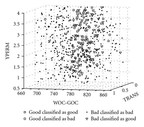
After the GP system completed 120 runs, the regression with the best classification accuracy was selected as the final proxy for the simulator. Table 4 gives the classification accuracy of this final solution: 82.54% on good models and 86.23% on bad models. The overall classification accuracy for the simulator proxy was 85.82%. Considering the length of the production data (30 years) to be matched and the quality of the data, this is a reasonably good classifier. Figure 12 shows the classification results in the parameter space defined by WOC-GOC, YPERM, and TRANS. It shows that the models with WOC-GOC outside the range of 750 and 825 were classified as bad models. Models with WOC-GOC within the range could be either good or bad depending on other parameter values.
| Good | Bad | Total | |
|---|---|---|---|
| Good | 82.54% | 17.46% | — |
| Bad | 13.77% | 86.23% | — |
| Total | — | — | 85.82% |
6.3. Interpolation and Interpretation
This GP classifier was then used to evaluate new sample points in the parameter space (step 7). For each of the 5 parameters (GOC-WOC was treated as 2 parameters), 11 samples were selected, evenly distributed between their minimum and maximum values. The resulting total number of samples was 115 = 161,051. Applying the GP classifier on these samples resulted in 28 125 being identified as good models while 132,926 were classified as bad models.
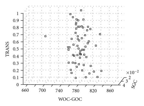
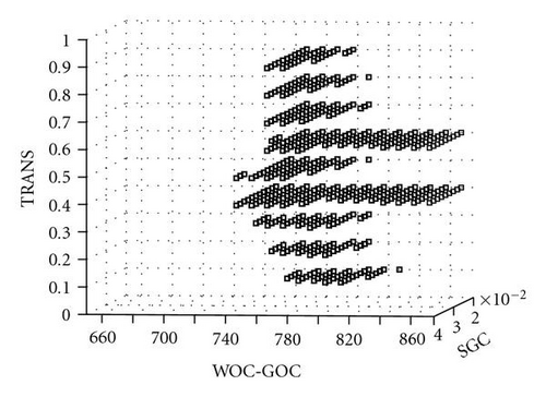
Figure 13 gives the 28 125 good models in the 3D parameter space defined by WOC-GOC, TRANS, and SGC. The pattern is consistent with that of the 63 good models identified by computer simulation, given in Figure 14.
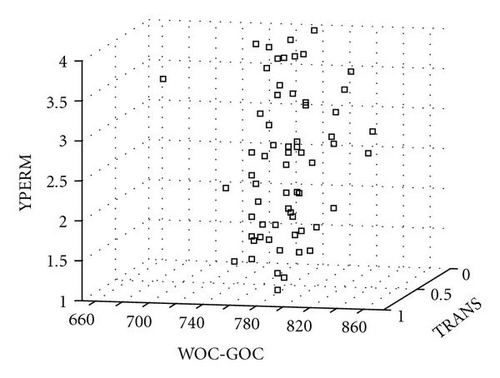
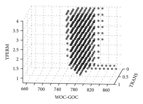
Within the 3D parameter space defined by WOC-GOC, YPERM, and TRANS, the good models have a slightly different pattern (see Figure 15). Yet the pattern is also consistent with the pattern of the 63 good models identified by computer simulation, shown in Figure 16.
Those results indicated that the GP classifier was a reasonable high-quality proxy for the full reservoir simulator. The 28 125 good models were then considered to be close to reality. Those models revealed the following reservoir characteristics of this West Africa oil field:
- (i)
the YPERM value was greater than 1.07;
- (ii)
the faults separating different geobodies (see Figure 6) were not completely sealing, indicated by the transmissibility values of good models are nonzero;
- (ii)
the width of the oil column (WOC-GOC) was greater than 750.
Meanwhile, we felt comfortable in using these 28 125 good models to forecast the cumulative gas injection in 2031 and estimate the forecast uncertainty accordingly (step 8). This work is reported in the following section.
7. Production Forecast Analysis
As mentioned previously, the forecast for oil production (or the volume of gas injection) also required computer simulation. Since it was not practical to make simulation runs for all 28 125 good models, a second simulator proxy was warranted. Similar to the way the history-matching proxy was constructed, we used GP to construct a second simulator proxy for production forecasting. In this way, production forecasts on these reservoir models can be estimated in a short period of time.
Since we had no knowledge about which of the 11 reservoir parameters has an impact on production forecast (The outliers study only investigated the correlation between reservoir parameters and the mismatch E, not the production forecast), all 11 parameters were used to construct the forecasting proxy. Also, the target forecast (F) was the cumulative volume of gas injection in the year 2031.
Unlike history-matching proxy, which is a classifier, production forecast proxy is a regression. The class imbalance issue therefore does not exist. Also, since all 581 computer simulation of production forecast data are good (only production data collected from the field are noisy), no data points need to be removed. The 581 data points were divided into three groups: 188 for training, 188 for validation, and 188 for blind testing. Training data was used for GP to construct the forecasting proxy while validation data was used to select the final forecasting proxy. In this way, overfitting is less likely to happen. The evaluation of the forecasting proxy was based on its performance on the blind testing data.
7.1. Experimental Setup
The GP parameter setup (see Table 5) was similar to the setup for outliers detection in Section 5. The only difference was that the fitness of an evolved regression is the MSE between simulator forecast (F) and regression output (R) of the 188 training data.
| Objective | Evolve a simulator proxy for production forecast |
|---|---|
| Functions | Addition, subtraction, multiplication, division, abs |
| Terminals | The 10 reservoir parameters listed in Table 1 plus oil column |
| Fitness | MSE: , F: simulator forecast |
| Selection | Tournament (4 candidates/2 winners) |
7.2. Results
The GP system continued for 120 runs and the regression with the smallest MSE on validation data was selected as the final forecasting proxy. Table 6 gives the R2 and MSE on the training, validation, and blind testing data. Since the proxy was to make predications for the next 30 years, which was a complex task, an R2 in the range of 0.76 was considered acceptable.
| Data Set | R2 | MSE |
|---|---|---|
| Training | 0.799792775 | 0.001151542 |
| Validation | 0.762180905 | 0.001333534 |
| Testing | 0.7106646 | 0.001550482 |
| All | 0.757354092 | 0.001345186 |
Figure 17 illustrates the crossplot for simulator and proxy forecasts on the 581 reservoir models. Across all models, the forecasting proxy gave consistent prediction as that by the computer simulator. Forecasting on the 63 good models (which are what are useful for decision making) is shown in Figure 18. In this particular case, the proxy gave a smaller forecasting range (0.12256) than that by the simulator (0.2158).
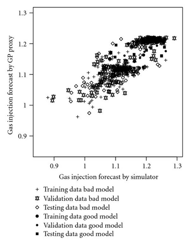
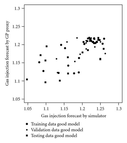
Similar to that of history-matching proxy, WOC-GOC was ranked to have the most impact on production forecasts. However, unlike the history-matching proxy, which only used 4 reservoir parameters (GOC-WOC, TRANS, YPERM, and SGC) to determine if a model was good or bad, the forecasting proxy used all 11 parameters to forecast production.
7.3. Forecasting Uncertainty Analysis
With the establishment of a good-quality forecasting proxy, we then used it to derive gas injection predictions from all good models identified by the history-matching proxy. Since each model selected by the history-matching proxy was described by 6 reservoir parameter values, there was freedom in selecting the values of the other 5 parameters not specified by the history-matching proxy. For each of the 5 unconstrained parameters, 5 sampling points were selected, evenly distributed between their minimum and maximum values. Each combination of the 5 parameter values was used to complement the 6 parameter values in each of the 28 125 good models to run the forecasting proxy. This resulted in a total of 28 125 × (55) = 87,890,625 models being sampled. Figure 19 gives the cumulative gas injection in year 2031, forecasted by these sampled models.
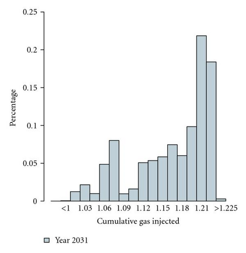

As shown, the gas injection range between 1.19 and 1.2 was predicated by the largest number of reservoir models (22% of the total models). This is similar to the predictions by the 63 computer simulation models (see Figure 20).
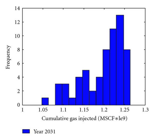
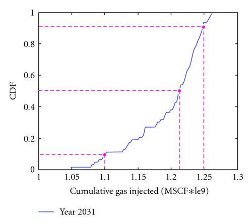
The cumulative density function (CDF) of the forecast proxy gave a P10 value of 1.06 trillion standard cubic feet (MSCF*le9), a P50 value of 1.18 MSCF, and a P90 value of 1.216 MSCF. This meant that the most likely (P50) injection volume would be 1.18 MSCF. There is a 90% probability that the injection volume would be higher than 1.05 MSCF (P10) and a 10% probability that the injection volume would be lower than 1.216 MSCF (P90). This uncertainty range allowed management in preparing for gas transportation and plan for other related arrangements.
Compared to the gas injection volume forecasted by the 63 good models identified by computer simulator, the uncertainty range was not much different; the difference between P10 and P90 was 0.15 in both cases. However, our results were derived from a much larger number of reservoir models sampled under a higher density distribution. Consequently, they provide the reservoir managers with more confidence to make business decisions accordingly.
8. Discussions of Execution Time
This case study consists of three phases: outliers detection, history matching, and production forecast analysis. In each phase, GP runs were conducted on a single Pentium CPU machine and took one weekend to complete. The total computer execution time is approximately 150 hours. Using the generated GP proxies, we were able to evaluate 161,051 reservoir models for history matching and 87,890,625 models for production forecasts. Without the GP simulator proxies, it would take the computer simulator 700 000 hours to process these reservoir models using a cluster machine with 124 CPUs. The GP overhead is well justified.
9. Concluding Remarks
History matching and production forecasting are of great importance to the planning and operation of petroleum reservoirs. Under time pressure, it is often necessary to curtail the number of computer simulation runs and make decisions based on a limited amount of information. The task is even more challenging when the reservoir has a long production history and the production data is unreliable. Currently, there is no standard way to conduct history matching for production forecasts in oil industry.
We have developed a method using GP to construct proxies for the full computer simulator. In this way, we can replace the costly simulator by the proxies to sample a much larger number of reservoir models and, consequently, obtain more information, which in turn, it is hoped, will lead to better reservoir decisions being made.
The case study on a West African oil field using the proposed approach has delivered very encouraging results.
- (i)
Although the reservoir has a significant history and noisy production data, we were able to construct a proxy which identifies history-matched models that have consistent characteristics with those matched by the full simulator.
- (ii)
By sampling a large number of reservoir models using the simulator proxy, new insights about the reservoir were revealed.
- (iii)
Production forecasts based on the large number of reservoir models gave management more confidence in their decision making.
- (iv)
These benefits were gained without introducing new computer simulation runs.
As far as we know, this is the first time such a method is developed to improve the quality of reservoir history matching and production forecasts. In particular, the innovative idea of casting the history-matching proxy as a classifier has allowed us to produce high-quality proxies which were unattentainable by other researchers who restricted their proxies to reproduce reservoir simulator response surface. We will continue this work by applying the method to other more challenging fields to evaluate its generality and scalability.
Acknowledgment
The authors would like to thank Chevron for the permission to publish these results.


