Automatic delineation of rational service areas and health professional shortage areas in GIS based on human movements and health resources
Abstract
How people travel to receive health services is essential for understanding healthcare shortages. The rational service areas (RSAs) are defined to represent local healthcare markets and used as the basic units to evaluate whether people have access to health resources. Therefore, finding an appropriate way to develop RSAs is important for understanding the utilization of health resources and supporting accurate resource allocation to the health professional shortage areas (HPSAs). Existing RSAs are usually developed based on the local knowledge of public health needs and are created through time-intensive manual work by health service officials. In this research, a travel data-driven and spatially constrained community detection method based on human mobility flow is proposed to automate the process of establishing the statewide RSAs and further identifying HPSAs based on healthcare criteria in a geographic information system (GIS) software. The proposed method considers the difference between rural and urban populations by assigning different parameters and delineates RSAs with the goal of reducing health resource inequalities faced by rural areas. Using the data in the State of Wisconsin, our experiment shows that the proposed RSA delineation method outperforms other baselines including the traditional Dartmouth method in the aspects of RSA compactness, region size balances, and health shortage scores. Furthermore, the whole process of delineating RSAs and identifying HPSAs is automated using Python toolboxes in ArcGIS to support future analyses and practices in a timely and repeatable manner.
1 INTRODUCTION
Health Professional Shortage Area (HPSA) designation identifies geographic areas or population groups with a shortage of healthcare services, including primary, dental, and mental health cares (HRSA, 2021b; Wang & Luo, 2005). The designation of HPSAs can help understand the spatial distributions and variations of health services, better allocate health resources and support policy making. It is important to make sure that the designated HPSAs can identify the greatest amount of the shortage areas so that limited health resources can be directed to people with the greatest needs.
The first step of the HPSA designation is to identify rational service areas (RSAs), which are then used as the input area units of HPSAs. The RSAs are relatively self-contained geographic units that represent people's travel patterns of seeking health services (Lopes, 2000). The RSAs are usually groups of census tracts, county subdivisions, an entire county, or multiple counties (HRSA, 2020a). Each state is required to develop its own statewide RSA plan that outlines the RSAs in a state/territory (HRSA, 2020b). To justify why a specific area is selected as an RSA, evidence of travel patterns, physical barriers or social-economic similarities should be provided (Lopes, 2000; Wang & Luo, 2005). However, there is no uniform approach to establishing the RSAs. Many of the RSAs are developed based on the local knowledge of public health needs and are created through time-intensive manual work by health service officials.
There has been much research working on the development of RSAs. Based on hospitalization records, the Dartmouth method was proposed in the 1990s to “assign zip code area into the town that contains the hospitals mostly used by the local residents” (Wennberg & Cooper, 1998). Jia et al. (2017) use a revised Huff model to delineate Hospital Service Areas (HSAs) based on the relationship between the hospital supply and patients' travel costs. In recent years, methods that apply the network theory have been proposed to model the patient discharge data in a spatial network where nodes are zip code regions and edges are hospitalization flows between these regions (Hu et al., 2018; Wang et al., 2021). Then the community detection approach is used to identify the strongly connected areas based on the hospitalization flows and those areas can then be used as RSAs (Newman, 2006). Some additional considerations such as the spatial constraints have also been incorporated into this process (Wang et al., 2021).
Although the above-mentioned methods have demonstrated their effectiveness in health service area delineation, there are still some issues that need further consideration. For example, the HPSA designation aims to address the resource shortage problem, which is mostly caused by the unequal spatial distribution of population and health providers (Liu, 2007). Studies have examined the recent trends in physician density and found a steady decrease of primary care physicians in more than half of rural counties from 2010 to 2017 (Machado et al., 2021). The trend indicates that providers tend to move from rural areas to urban areas, probably because there are more potential patients in the population-dense area. The uneven spatial distribution of healthcare providers creates barriers to access health services, especially for rural area residents and it leads to potential health disparities. Therefore, rural/urban residents may generate significantly different visit patterns to health providers, and such differences should be considered in the development of the health service areas.
To fill the gap in the current research, we propose a travel data-driven and spatially constrained community detection method that considers different characteristics and constraints of rural and urban areas to automate the delineation of RSAs and HPSAs (i.e., Auto-RSA-HPSA) based on healthcare criteria in a geographic information system (GIS) environment. The general workflow is shown in Figure 1. By incorporating the urban/rural population threshold into the spatial network-based community detection algorithm, our method is adjustable based on the rural population percentage to account for the health access inequality. In addition, it has been realized by public health officials that a method that can be conducted automatically, adapted to different areas and evaluated by quantitative measurements is needed in the designation process. This study develops a completely automated process for the establishment of RSAs and the delineation of HPSAs in GIS. We first propose a mobility data-driven and spatially constrained community detection method based on human mobility flow data collected from anonymous mobile phones to establish the statewide RSAs. Then, the generated RSAs are evaluated through multiple criteria including both spatial and non-spatial aspects to identify the HPSAs. The results are measured using health-related metrics and the performance is compared with the traditional Dartmouth method. This study intends to provide insights into the use of human mobility data and health-related metrics, network analysis, and GIS automation workflow that can help the state health departments to develop candidate plans for RSAs and HPSAs in primary, dental, and mental care.
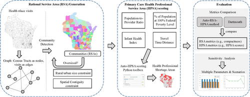
The remaining sections of this paper are organized as follows: we first review the related literature in Section 2. We then introduce the datasets used in this research and the proposed spatially constrained community detection method in Section 3. We then present the result evaluation and sensitivity analyses in Section 4. Finally, we conclude our study and share some directions for future work in Section 5.
2 LITERATURE REVIEWS
2.1 Rational/Hospital Service Area development
One of the most widely used methods for HSA development is the Dartmouth method proposed by the Dartmouth Institute for Health Policy and Clinical Practice in the United States (Wennberg & Cooper, 1998). Based on the Medicare hospitalization records that indicate how patients travel from their ZIP Code to seek health services, this method defines HSAs to represent community-based local healthcare markets and Hospital Referral regions (HRRs) to represent regional healthcare markets for tertiary medical care (Wennberg & Cooper, 1998). Following the traditional Dartmouth method, a primary care service area method was also developed using only the Medicare data for primary care physicians (Goodman et al., 2003).
- The hospitals are collected and assigned to the city/town where they are located at.
- Based on the Medicare hospitalization data between the hospital and the patients' zip code area, each zip code is assigned to the town containing the hospital that mostly used by the residents in the zip code area.
- Visual examinations are conducted to ensure the shapes are contiguous and the final HSAs are determined.
The original Dartmouth method has been used by many states for delineating HSAs in the United States (Jia et al., 2015). However, researchers have also realized that there are some issues with the original Dartmouth method. First, it was developed using the Medicare data, which only includes certain types of patients (e.g., people over the age of 65). Therefore, the results may not be representative of other types of population (Hu et al., 2018; Wennberg & Cooper, 1998). Second, the last step of the Dartmouth method involves visual examination and introduces uncertainties into the result as the designation may be arbitrary (Hu et al., 2018; Wang et al., 2021). Third, the health service markets are dynamic and have changed over time, but the results of the Dartmouth method have been static since its proposal (Wennberg & Cooper, 1998).
To solve those problems, multiple researchers have worked on improving the Dartmouth method in different ways. Klauss et al. (2005) developed a Swiss method similar to the Dartmouth method using the hospital discharge records for all patients. This method was also population-based by using a small area analysis at the census level and can accurately describe the differences across regions with homogeneous population groups (Klauss et al., 2005). Following that, a Dartmouth-Swiss hybrid method was used to compare the temporal variations of Medicare-derived HSAs over the two decades (Jia et al., 2015). The study found that the boundaries of the HSAs have been significantly changed and are not representative of the whole population (Jia et al., 2015). To provide a more solid result, the authors applied the Huff model to re-demarcate the HSAs by assuming that the probability of visiting a hospital is positively related to the number of beds and negatively related to the travel distance (Jia et al., 2015). The Huff model method was further improved by designing the distance decay function based on the actual hospitalization travel patterns (Bai et al., 2023; Jia et al., 2017). However, the Huff model may oversimplify the visit patterns of seeking health services as there are many other factors affecting whether people would visit a hospital, for example, the specialties of physicians or people's work location. A refined Dartmouth method that requires hospitalization data was also developed, where the authors resolved some uncertainties in the original method and developed a standardized delineation approach that can be automated in a GIS tool (Wang & Wang, 2022).
Despite there exist other improved Dartmouth methods, all these existing methods are based on hospitalization data, and such data are usually not available to the public nor to researchers. There is a need to delineate RSAs based on travel patterns using openly accessible human mobility data.
2.2 Spatial networks and community detection
Another major innovation in Health Service Area delineation was inspired by the network theory, which models the visit flows from patients to health providers in a spatial network (Hu et al., 2018; Wang et al., 2021). Specifically, the approach named community detection aims to identify strongly connected communities based on the movement flows in the network, and those communities can then be used as RSAs (Newman, 2006). With the goal of maximizing the hospital visit flows within each community and minimizing the flows between communities, this approach divides regions based on their interactions and reveals the hidden relationship among areas (Hu et al., 2018; Newman, 2006). Hu et al. (2018) first used the Louvain community detection method to extract HSAs and HRRs in Florida based on the state inpatient database. Pinheiro et al. (2020) further conducted a comparative analysis of different community detection algorithms on Health Service Area delineation. To incorporate the spatial component into the traditional algorithm, Wang et al. (2021) designed spatial-constrained community detection methods to enforce the spatial contiguity of the results. Compared with traditional health service area designation methods, the community detection method has the following advantages: first, it is based on complex network theory and has solid theoretical support; second, it can be automated for repeatable implementation; and lastly, it is computationally efficient (Pinheiro et al., 2020; Wang et al., 2021; Wang & Wang, 2022).
All of the existing studies introduced the use of patient-hospital discharge data to extract the health/hospital/rational service areas. However, access to hospitalization data is very limited due to privacy concerns, and such data may not be available for many low-income and middle-income areas, which affects the scalability of the existing methods (Jia et al., 2015). In addition, the existing hospital visits may not reflect the potential needs for new hospitals/clinics. Therefore, we will explore additional data sources including population-scale aggregated travel patterns to provide potential insights for the development of RSAs and HPSAs in this research.
3 METHODS
3.1 Data and study area
The study area of this research is the State of Wisconsin in the United States. It is bordered by Lake Superior to the north, Michigan to the northeast, Lake Michigan to the east, Illinois to the south, Iowa to the southwest and Minnesota to the northwest (Martin, 1965).
This study uses the SafeGraph business venue database and place visit patterns (SafeGraph, 2023) as its main data source. SafeGraph collects over 8 million points of interest (POIs) with visit patterns in the United States. The POIs are classified based on the North American Industry Classification System (NAICS) 6-digit sector codes. We selected three categories of interest: 621—Ambulatory Health Care Services, 622—Hospitals and 446,110—Pharmacies and Drug Stores as we are only interested in visits to health-related places. The health shortage designation plans require the use of the same RSA geographic unit but different HPSA scoring criteria for three healthcare types (primary care, mental care and dental care) according to the Shortage Designation Manual (HRSA, 2021b). Therefore, the visit flows to all types of healthcare services are used to develop the RSAs. The fine-resolution visit patterns to those POIs were collected from anonymous smartphone users and were aggregated to census block group level for privacy preservation. The aggregated visit data is from about 10% devices in the United States and the data sampling has been illustrated to be highly correlated with the U.S. Census populations (Kang et al., 2020). The visit data from census block groups to all health-related POIs are further aggregated to the census tract level as such coarser-resolution data are openly accessible and it is a sufficient spatial resolution to understand the mobility interactions and delineate RSAs, as most of RSAs have similar sizes with counties. The origin census block group is aggregated to the census tract containing it, and the destination POIs are also aggregated to the census tract in which they are located. So the data becomes the origin–destination flows at the same spatial resolution. The time window used in this study was from August 2021 to October 2021.
The health providers' information including locations, full-time equivalent (FTE) and specialty are provided by the Wisconsin State Primary Care Office. The FTE means a provider's working hours divided by the hours for a full-time workweek, so if a provider works 40 h a week, her/his FTE is 1. Other data sources include the U.S. Census American Community Survey (ACS) 5-year estimates, and the Centers for Disease Control and Prevention (CDC) Period Linked Birth/Infant Death File 2014–2018.
3.2 Community detection method
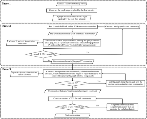
The RSA generation workflow with three phases in this study is shown in Figure 2. The method is built on spatial network-based community detection algorithms with multiple iterations and additional constraints designed for the targeted problem. More details are presented in the following sections.
3.2.1 Community detection algorithms
The random walk, Louvain, and Leiden community detection algorithms are adopted and integrated with our GIS workflow in this study given their popularity and scale flexibility characteristics. The GIS framework supports the selection of a different community detection algorithm that works the best for different area delineation use cases.
The random walk algorithm was proposed with the basic idea that short random walks tend to be ‘trapped’ in the same community in a network (Pons & Latapy, 2005). It uses a structural similarity to represent the distance between nodes and between communities. The distance is calculated based on the transition probability of moving from one node to another in a single step. This approach is a hierarchical clustering algorithm that groups nodes in the network iteratively into communities (Pons & Latapy, 2005). At the initial stage, every node (i.e., census tract in this study) is a single community, and the distances based on the structural similarity between all adjacent nodes are computed. Two communities will be chosen based on the distance measure and merged into a new one, and then the distances among new communities will be updated until there is only one community of all nodes. The algorithm captures much information on the community structure and is computationally efficient. However, the performance can vary based on the network's size and structure.
The Louvain algorithm was proposed by Blondel et al. (2008) as a popular method to extract communities based on modularity optimization. The modularity is used to measure the quality of the communities. It compares the fraction of edges that fall within the communities to a null network with edges placed randomly (Newman, 2006). The modularity ranges from −1 to 1 and is larger when the division result has more within-community edges. In other words, a larger modularity means the nodes with stronger connections are better grouped together. Exact modularity optimization is NP-hard, and the Louvain algorithm uses a heuristic method to identify high modularity partitions (Blondel et al., 2008). The algorithm has two phases: initially, each node is considered as a single community, and the method calculates the modularity gain by moving each node to its neighbor's community, then the node will be placed in the community with the maximum gain (Blondel et al., 2008). This process is repeated until there is no modularity improvement. Then, in the second phase, the algorithm builds a new network where the nodes are the communities from the first phase and the first phase can be reapplied to this new network. The Louvain algorithm has been proven to be intuitive, and easy to implement. It runs very fast and can identify communities with good quality in large networks (Blondel et al., 2008). However, it suffers from a resolution limit that may prevent it from identifying small-size communities.
The Leiden algorithm is a recent improvement on the Louvain algorithm. It was found that the Louvain algorithm may generate disconnected communities, and the Leiden algorithm was proposed with better partitions that all communities are internally connected (Traag et al., 2019). It has three phases: (1) moving node locally, (2) refining the partition and (3) aggregating the network. In the first phase, Leiden uses a fast local move procedure that only visits nodes whose neighborhood has changed. During the refinement phase, each community generated from the first phase is evaluated to make sure it is strongly connected and may be split into subcommunities. The Leiden algorithm has outperformed the Louvain algorithm in practical applications in terms of speed and the quality of the results (Traag et al., 2019).
One important characteristic of the above methods is that they are scale flexible (Blondel et al., 2008; Hu et al., 2018; Pons & Latapy, 2005; Traag et al., 2019). Each process generates a hierarchical structure and allows the examination of all hierarchical levels to select the most appropriate community structure for the use case. This property is very helpful for real-world planning as one may want to compare results at different scales to understand the scale effects. For example, to support the analysis of the Modifiable Area Unit Problem (MAUP) in geography (Openshaw, 1984).
The health-related place visit flows at the census tract level will be used as inputs to the community detection algorithm. As shown in Figure 2 Phase 1, the census tract are the nodes, the edges are health-related visits, and the edge weights are the intensity of flows. The generated hierarchical community structure will be evaluated at multiple levels to select the best community structure as the RSAs.
3.2.2 Population constraints
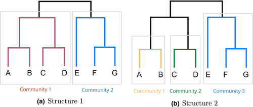
To evaluate the appropriate geographic scale of RSAs, one needs to understand how the size of an RSA is determined and measured. There are multiple aspects that affect the size of RSAs, for example, how populations are distributed across space, their demographic and socioeconomic status, and how people move around in their surrounding areas (Lopes, 2000). The most straightforward criterion that measures the scale of RSAs is population. One strict guidance of the shortage designation is that the population in the RSAs should not exceed 250,000 (HRSA, 2020a). However, this universal upper population limit is not very powerful as the size of one RSA is always smaller than this threshold in practice. To better use population limit to guide the RSAs scale selection, different population thresholds will be examined to select the appropriate RSAs sizes in the community structure hierarchy. More specifically, the population threshold (max pop) is used as the upper population limit of the RSAs. In case the current result has RSAs over this population limit, one will go down a level in the hierarchical structure to select a finer scale of RSAs. An example is shown in Figure 3. The structure 1 has two communities, if community 1 is over the population threshold, it will be further split into its next hierarchy, generating structure 2 on the right side.
While population is an effective criterion to determine the RSA sizes, it is always a uniform threshold across the whole study area. However, people are not evenly distributed across the space and neither are health resources. In particular, rural and urban populations can have significantly different travel patterns to visit health providers (Luo, 2004). In rural areas, people need to travel further due to the sparsity of the health providers, while the urban population has relatively easier access to the providers. When the population limit is uniform, it will lead to significantly different areal sizes for RSAs in rural and urban areas. Given the same population constraint, rural areas tend to form a larger community than urban areas due to the low population density. However, this can lead to disadvantages for rural areas as they have to travel further to receive health resources with larger areal sizes (Hart et al., 2002). In addition, there exist small areas with high needs for health resources, but once they are grouped with other areas into a larger-area RSA, their shortage cannot be identified. To address this problem, different population parameters are adopted in the RSA development to reduce the inequalities between rural and urban areas. The goal is to make sure that areas with large area sizes but low population density (such as some rural census tracts) can receive enough attention.
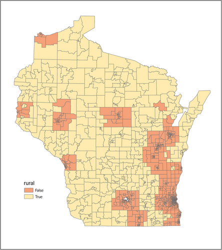
In summary, we adopt different population constraints to rural and urban areas in the RSA development. When multiple census tracts are grouped as an RSA, a rural population percentage is calculated. If the percentage exceeds a pre-defined value (e.g., 50%), the RSA is considered as a rural RSA and rural constraints are applied; otherwise, urban constraints are used. The rural and urban population definition is provided by the Health Resources and Services Administration (HRSA) (HRSA, 2021a). It combined the rural area definitions from the United States Census Bureau and the Office of Management and Budget, and incorporated that with Rural–Urban Commuting Area codes to create their own definition. The final rural areas are defined at the census tract level. Figure 4 shows the spatial distribution of rural and urban census tracts in the State of Wisconsin.
In addition to population, the maximum number of census tracts (max CTs) in an RSA is jointly used as a constraint to ensure more stable results. Depending on the rural population percentage in each RSA, the population and census tract constraints are different. We tested different parameter settings in our experiments (more details in Table 5). The RSAs with population and number of census tracts larger than the upper constraints will be selected and further split.
The process is implemented as Phase 2 in Figure 2. In each iteration, the community detection method is conducted first to generate the optimal communities. The rural population percentage is calculated to decide whether each community is considered as rural or urban, and be assigned with corresponding split parameters. Then the communities are evaluated based on the population and census tract number constraints to determine if they need to be further split. If they need to be split, the community is sent back to the community detection algorithm to be split into its lower hierarchy.
It should be emphasized that the creation of RSAs in no way implies that residents must seek and obtain services within their areas. The purpose of defining RSAs is to analyze health-related travel patterns and to identify gaps in health resource allocation planning.
3.2.3 Spatial constraints
After the implementation of the community detection algorithm with the population constraint, the whole area is split into a set of communities (i.e., candidates of RSAs). However, the division cannot always be used immediately because the spatial relationship of geographic units is not directly considered in the community detection method and may lead to some disconnected or isolated communities. To solve this problem, geographic adjacency is used to enforce spatial contiguity by cutting disconnected communities and merging small communities with their neighboring communities.
First, we need to find all communities that are not spatially contiguous, and this is implemented by building a subgraph for each generated RSA based on the spatial adjacency matrix and looking for the minimum cut in each subgraph. The minimum cut is the minimum total weight of edges that need to be removed to separate the graph into two components (Stoer & Wagner, 1997). If the graph is already not spatial contiguous, the minimum cut will be 0 and this indicator can help find all the disconnected RSAs. The approach can support the automatic identification of non-contiguous RSAs and is very helpful especially when one has a large number of regions to analyze.
After cutting all the non-contiguous RSAs, the remaining problem is to merge the small and isolated RSAs with their neighboring RSAs. In Phase 3, a threshold of census tract count is used to determine the size of small RSAs (e.g., if an RSA has only two census tracts, it is considered as a small RSA in this study). In the merging process, each small RSA or isolated RSA will go through an iteration, where it will be merged with each of its neighbor RSAs and the global modularity will be re-calculated after the merge. The RSA will finally be merged with the neighbor RSA that can generate the maximum modularity.
Figure 5 shows an example of enforcing the spatial constraint in our algorithm. Without considering spatial contiguity, the purple color community, number 89, is disconnected as shown in Figure 5a. So is the blue community, number 91. In addition, the orange community, number 43, is an isolated census tract surrounded by another community 42. The disconnected communities 89 and 91 are first cut into separate ones, with part of them being considered as small isolated communities that need to be merged. The small communities are then identified and merged into their neighboring communities. Figure 5b shows the result after the cut-merge steps; the remaining four communities are all spatially contiguous.
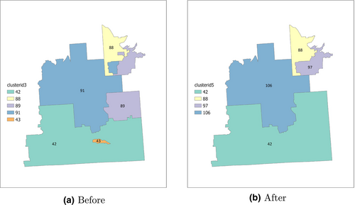
The Phase 3 in Figure 2 describes the process of enforcing the spatial constraint. The min-cut of each community is calculated first to identify and cut the non-contiguous communities. The small communities are then merged into neighbor communities. The final communities are obtained after these two steps.
3.3 Evaluation metrics
Two aspects are considered to measure the RSA performance using our proposed method. The first part focuses on the RSA shapes and its components, and the second part focuses on the health shortage areas identified based on RSAs.
3.3.1 RSA measures
The evaluation of RSAs focuses on the division result of community detection, specifically on the geographic structures of generated communities. The following metrics are used.
The balance in region sizes measures the evenness of several aspects across RSAs such as the number of census tracts, population, and providers. A more balanced distribution of numbers across all RSAs means that they are more equally representative of the whole region and the variances of RSAs are small.
3.3.2 HPSA scoring
Besides the RSA structure evaluation, one important application of RSAs is that they are used as the basic units for Health Professional Shortage Areas (HPSAs) designation. The providers in the HPSAs will receive incentives or financial assistance to support them in better serving the shortage areas (Luo, 2004). To understand the performance of developed RSAs, the Primary Care Geographic HPSAs are identified based on four criteria used in the Shortage Designation Management System (HRSA, 2020a). The population-to-provider ratio, the percentage of the population at 100% Federal Poverty Level, the infant health rate, and the travel time or distance to the nearest non-designated provider are calculated and scored. We collected the demographic information required to calculate the population-to-provider ratio and percent of individuals below 100% of the federal poverty level through the U.S. Census Bureau. The infant health index is calculated based on the infant mortality rate and low birthweight rate, and the data is collected from the Centers for Disease Control and Prevention (CDC). The travel time/distance is calculated based on the locations of providers using ArcGIS “Find nearby locations” tool. The final HPSA score for primary care is a weighted sum of the four criteria (i.e., 2*population-to-provider ratio + population poverty rate + infant health index + travel time) and is calculated for each RSA. A higher HPSA means that the area is under a greater shortage of providers. More details about how HPSAs are finalized can be found in the HPSA designation manual (HRSA, 2020a).
After establishing HPSAs in the study area, the number of HPSAs, the population covered by HPSAs, the population-to-provider ratio in HPSAs and the average HPSA scores are used as HPSA evaluation metrics. Given a certain RSA plan, the HPSA scores are generated, and the identified HPSAs are evaluated. A Python toolbox in ArcGIS is also developed to support the automation of the RSA generation and HPSA designation process.
4 RESULTS
4.1 Community detection
Five scenarios are implemented to compare the performance: (1) the proposed Auto-RSA-HPSA method with rural/urban constraints using the random walk algorithm, (2) the proposed Auto-RSA-HPSA method with rural/urban constraints using the Louvain algorithm, (3) the proposed Auto-RSA-HPSA method with rural/urban constraints using the Leiden algorithm, (4) the proposed method with only a population constraint of 250,000 using the random walk algorithm (abbreviated as random walk baseline), and (5) the traditional Dartmouth method.
The number of derived RSAs for the five scenarios, the rural/urban constraint parameters, and their average running time over ten iterations are listed in Table 1. The random walk, Louvain and Leiden represent the proposed Auto-RSA-HPSA method implemented using the corresponding algorithm, respectively. The number of RSAs is closely related to the selection of rural/urban parameters. The optimal rural/urban parameters of Scenario 1 using the random walk algorithm are selected based on the sensitivity analysis that will be introduced later. Scenario 2 and 3 parameters are selected in order to generate a similar number of RSAs as Scenario 1 so that their scales are comparable. Scenario 4—random walk baseline uses the proposed Auto-RSA-HPSA method with only a population constraint of 250,000. Therefore, the number of RSAs from the random walk baseline is fewer than that of the previous scenarios because of the population constraint. The original Dartmouth method result is obtained from the official website of Dartmouth Atlas project (Wennberg & Cooper, 1998). The execution times of the scenarios are relatively similar, and the Auto-RSA-HPSA method using random walk requires a slightly longer execution time than the rest of the scenarios.
| Scenario | 1 | 2 | 3 | 4 | 5 |
|---|---|---|---|---|---|
| Method | Random walk | Louvain | Leiden | Random walk baseline | Dartmouth |
| Number of RSAs | 164 | 169 | 165 | 70 | 100 |
| Rural population | 20,000 | 40,000 | 40,000 | 250,000 | N/A |
| Urban population | 40,000 | 70,000 | 70,000 | 250,000 | N/A |
| Rural census tracts | 3 | 6 | 6 | 0 | N/A |
| Urban census tracts | 10 | 18 | 18 | 0 | N/A |
| Execution time (s) | 59.2 | 54.5 | 54.7 | 54.7 | N/A |
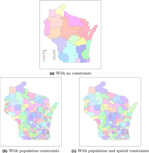
The result of the Auto-RSA-HPSA method with the random walk algorithm (Scenario 1) is used as an example to illustrate how the RSAs are derived step by step. The initial derived RSA result from the random walk algorithm is a global optimal result when the maximum modularity is reached without any additional constraints. The result map is shown in Figure 6a, where in total there are 18 communities with each census tract colored according to its community membership. Based on the urban/rural constraints in Table 1, and the rural/urban population ratio threshold of 0.5, all 18 communities are selected to be further split. This process iterates until all communities fulfill the population constraints. The result after the splits is shown in Figure 6b. There are 205 communities in total and the communities (i.e., RSAs) become much smaller compared with Figure 6a. Then, the spatial contiguity constraint is enforced to cut and merge the communities. The final result of the community detection is shown in Figure 6c. The number of final communities is 164. Compared with the results before the spatial contiguity constraint step, many small communities are merged with nearby communities.
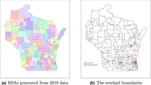
To ensure that the data in the selected time range (August–October 2021) are representative, we also collected an additional 1-year data in 2019. The origin–destination flow matrices of these two periods have a high structure similarity of 0.94 (Jin et al., 2020). In addition, we implement the same method in Scenario 1 using the 2019 data and the generated RSA results are compared with results using the Aug-Oct 2021 data. As shown in Figure 7a, using the data from 2019, the Auto-RSA-HPSA method using random walk generates 162 RSAs. The data from 2021 generates 164 RSAs and is on Figure 6c. By visual examination, many RSAs are identical in both results or have similar shapes. We then overlay the two RSA results together using different boundary colors (Figure 7b), and most of the boundaries are the same with a few differences. Therefore, we conclude that the selected 3-month data result is representative enough to be used in our case study. We suggest that when the method is implemented for practical applications in other regions, one may keep updating the mobility data regularly to obtain the most up-to-date human mobility data-driven RSA delineation results.
4.2 RSA evaluation
Besides the visual comparison, multiple quantitative metrics are computed for the five scenarios to evaluate the quality of RSAs.
4.2.1 Geographic compactness
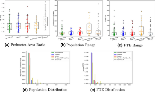
The PAC ratio measures the regularity and the compactness of the shapes. As shown in Figure 8a, the RSAs derived by the proposed Auto-RSA-HPSA method using random walk, Louvain and Leiden have very similar PAC values and their interquartile range (represented by the black rectangle) are lower than that of the random walk baseline and the Dartmouth method. The RSAs from Scenario 1—random walk and Scenario 3—Leiden have slightly lower median PAC values (represented by the orange line) than that of Scenario 2—Louvain algorithm. The RSAs from Scenario 4—random walk baseline have a larger median PAC value compared with the Auto-RSA-HPSA methods' results and the RSAs from the Dartmouth method have much larger PAC values. The small PAC values in Scenarios 1, 2 and 3 indicate that our proposed Auto-RSA-HPSA methods with rural/urban constraints generate more regular and consolidated shapes, which is more favorable in RSA development.
4.2.2 Balance in region sizes
The balance in region sizes is measured using the population in each RSA and the total providers in each RSA, represented by the full-time equivalent (FTE). The box plots of the population distribution in each scenario are shown in Figure 8b and the standard deviation is also calculated and shown in the x-axis labels. The data for the proposed methods using random walk, Louvain, and Leiden are generally more concentrated and have smaller values than the other two scenarios. Scenario 4 using the random walk baseline method has widely distributed data values. For Scenario 5 of the Dartmouth method, although there are data distributed at the bottom of the box plot, it also has a few outlier values that go beyond the whisker range, some of the outliers are over 350 thousand and removed from the figure. For the population standard deviation, the results from Scenarios 1, 2, and 3 have much smaller standard deviations than the results in Scenarios 4 and 5. Among the first three scenarios, the RSAs from the Leiden algorithm have the smallest population standard deviation. The random walk baseline using only a population limit of 250,000 has the second-largest standard deviation. The Dartmouth method yields the greatest standard deviation. Figure 8d shows the histogram of the same population data, it is clear that the proposed methods using random walk, Louvain, and Leiden represented by the green, blue, and red bars are heavily right-skewed because of their small RSA sizes. Most of the data are distributed in the first bin. Figure 8c shows the box plot of the provider FTE. For the proposed methods using random walk, Louvain and Leiden, the data are mostly distributed near the bottom of the box plot. This is also reflected by the histogram of the FTE data in Figure 8e: data of Scenario 1, 2, 3 are heavily right-skewed. The FTE standard deviation shows similar trends as the population standard deviation, with the proposed Auto-RSA-HPSA methods yielding the smallest standard deviations and the Dartmouth method having the greatest standard deviation. The RSAs from the Auto-RSA-HPSA method using the Louvain algorithm have the smallest FTE standard deviation. The smallest standard deviations of population and FTE distribution indicate that the proposed methods generate more equally distributed regions, and the RSAs are more balanced in terms of population and provider distributions.
4.3 HPSA delineation and scoring
The five scenarios of RSAs are then used to further identify HPSAs, which include primary care, dental care, and mental healthcare providers but with different criteria. In this paper, we only demonstrate the effectiveness of our proposed Auto-RSA-HPSA method using the primary care provider data while we have done the analyses for all the care types in collaboration with the Wisconsin Department of Health Services. Figure 9 shows the final HPSAs for the five scenarios, where the blue-shaded regions are Primary Care Geographic HPSAs. From the visual examination, the first three scenarios of the proposed methods with rural/urban constraints have greater HPSA coverages than the remaining two scenarios. The distribution of HPSAs for Scenarios 1, 2 and 3 are similar but with small differences. On the northern part of the study area, the area sizes of the HPSAs tend to be large, and on the southern part the HPSA areas become smaller. Based on Figure 4, most of the northern part of the study area is defined as rural areas. The difference in area sizes reflects one goal of the proposed framework: people in rural and urban areas have different travel patterns to receive health services, and this difference should be reflected in the RSAs.
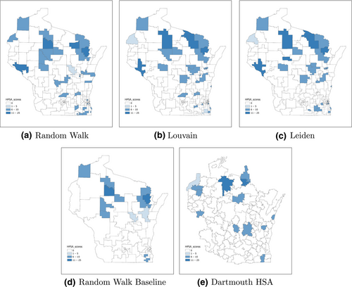
Table 2 shows the statistics of the HPSAs including the number of HPSAs, total population and providers Full-Time Equivalent (FTE) covered, the population-to-provider ratio and the average HPSA scores. We first compare Scenarios 1, 2, 3, as they represent the proposed Auto-RSA-HPSA method with different community detection algorithms. Scenario 1 with the random walk algorithm generates the greatest number of HPSAs. For the total population covered by HPSAs, the HPSAs from Scenario 3 using the Leiden algorithm cover the maximum population of 804,277, which is significantly more than that of other scenarios. The population covered by the HPSAs from Scenario 1 using the random walk algorithm is a little more than that of Scenario 2 using the Louvain algorithm. For the number of providers covered by the HPSAs, we measure it using the full-time equivalent of providers. Among Scenarios 1–3, the HPSAs derived from Scenario 3 using the Leiden algorithm cover the least amount of providers. The following metric, the population-to-provider ratio measures the provider shortage. It reflects on average how many people visit the same provider. The HPSAs from Scenario 3 using the Leiden algorithm have the highest ratio of 7018.1, meaning that the HPSAs are under the greatest provider shortage compared with that in Scenario 1 and 2. Scenario 3 using the Leiden algorithm also has the highest average HPSA scores, and Scenario 1 and 2 have the same second highest score.
| Scenario | 1 | 2 | 3 | 4 | 5 |
|---|---|---|---|---|---|
| Method | Random walk | Louvain | Leiden | Random walk baseline | Dartmouth |
| Number of RSAs | 164 | 169 | 165 | 70 | 100 |
| Number of HPSAs | 36 | 32 | 34 | 12 | 13 |
| Population | 744,681 | 739,796 | 804,277 | 412,464 | 218,872 |
| Provider (FTE) | 125.5 | 121.1 | 114.6 | 100.9 | 46.7 |
| Population: FTE | 5932.5 | 6111.5 | 7018.1 | 4086.8 | 4686.8 |
| Average HPSA score | 9.4 | 9.4 | 10.2 | 8 | 8.6 |
We then compare Scenario 1–3 with Scenario 4 and Scenario 5. Scenario 4 using the proposed framework with a population constraint of 250,000 identifies 12 HPSAs out of 70 RSAs, which is the fewest HPSAs of all scenarios. In addition, HPSAs from Scenario 4 have the lowest population-to-provider ratio as well as the lowest HPSA score. Scenario 5 using the Dartmouth method has 13 HPSAs out of 100 RSAs. The HPSAs identified from Scenario 5 cover the fewest amount of population with the second lowest population-to-provider ratio. The HPSA score is also lower than that of the first three scenarios.
In summary, the proposed Auto-RSA-HPSA methods with rural/urban constraints can outperform other baselines in the number of HPSAs, the level of HPSA shortage and the average HPSA score. The proposed Auto-RSA-HPSA method using the Leiden algorithm has the best performance in HPSA metrics among the three community detection algorithms. However, it is worth noting that we are not arguing that one specific community detection method can outperform other community detection methods in all use cases, rather we consider there is flexibility of selecting a community detection method in our integrated GIS framework, where one can select the method (or extend using their own preferred method) that works the best for their area delineation use case.
4.4 Sensitivity analysis
Two parts of the proposed method require parameter setting. The first one is the rural population percentage threshold that decides whether an RSA is considered as rural or urban. The second part is the rural/urban constraints including the population and the number of census tracts that affect whether an RSA should be further split or not. The sensitivity analysis is conducted to understand the effect of those parameters on the results using the Auto-RSA-HPSA method with the random walk algorithm.
4.4.1 Rural population percentage threshold
In the process of RSA development, whether an RSA should be assigned the rural or the urban parameters depends on the percentage of the rural population. If the rural population percentage is above the pre-defined threshold, rural parameters are applied; otherwise, urban parameters are applied.
This percentage threshold can vary across regions and affect the final RSA development. To understand and quantify the effects of this threshold, a range of rural population percentages are selected to generate the RSAs. As the ultimate goal of RSA development is to identify areas with healthcare shortages for future resource allocation, the performances are measured primarily based on the HPSAs that can be identified from the results. The number of HPSAs, the rural and urban populations covered by HPSAs, and the amount of providers in the HPSAs are calculated as evaluation metrics.
As shown in Table 3, the number of RSAs and HPSAs generated from different thresholds are almost the same, with a slight change for thresholds 0.7 and 0.8. The results for rural and urban populations covered by HPSAs are shown in Figure 10a, where from threshold 0.2 to 0.6, the results are relatively stable. The rural population (represented by the orange bar) drops at thresholds 0.7 and 0.8. Compared with previous thresholds, a higher rural population percentage threshold will make more areas be defined as urban, and be assigned with urban parameters. This can affect the final numbers and shapes of RSAs and HPSAs. At threshold 0.8, both the rural population and the urban population are lower than the result of the remaining thresholds. Figure 10b shows the providers covered by the HPSAs. Similar to the population trend shown in Figure 10a, the number of FTE of the HPSAs is stable for a threshold from 0.2 to 0.6. The total FTE starts decreasing at threshold 0.7 and reaches its lowest value at threshold 0.8.
| Rural population threshold | 0.2 | 0.3 | 0.4 | 0.5 | 0.6 | 0.7 | 0.8 |
|---|---|---|---|---|---|---|---|
| Number of HPSAs | 36 | 36 | 36 | 36 | 36 | 34 | 34 |
| Number of RSAs | 165 | 164 | 164 | 164 | 164 | 163 | 163 |
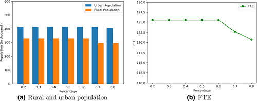
In summary, when the rural population percentage threshold changes from 0.2 to 0.8, the numbers of RSAs and HPSAs are very stable. There are some variances for population and providers covered, but the results are generally stable, especially between the range of 0.2 to 0.6. The threshold of 0.5 is used in the proposed method presented above.
4.4.2 Rural/urban population constraints
As mentioned above, the population constraint is applied to determine whether an RSA should be further split and this constraint is different for rural and urban areas. The selected population and census tract thresholds can affect the desired community scales. According to the National Shortage Designation Process in the U.S. (HRSA, 2020a), a whole county is considered rational for an RSA with no further justification. The counties have been frequently used as RSAs by state officials from the Department of Health Services in Wisconsin. Therefore, we selected the population thresholds based on the population statistics of counties in Wisconsin in Table 4. We used the 25% and 75% of the population percentiles as the approximate range of our population threshold to ensure that the final RSAs derived from our proposed method have a similar size with counties in Wisconsin. Our method can take different parameter values as the inputs of the Python tools embedded in a GIS environment, which enables users from other States to select their preferred population thresholds.
| Min | 25% | 50% | 75% | Max |
|---|---|---|---|---|
| 4254 | 18,773 | 39,336 | 84,304 | 929,362 |
Multiple sets of parameters are selected to examine their effects on the final RSAs and HPSAs for the proposed Auto-RSA-HPSA method using the random walk algorithm (Table 5). Generally, the rural parameters are smaller than the urban parameters so that rural areas can have finer-resolution RSAs. Take Case 1 as an example, if there is an RSA with 60,000 population and 15 census tracts in urban areas, it would remain the same RSA; but if it is in rural areas, it should be split because it meets the constraint of rural areas. Case 3 has the same parameters for rural and urban areas, and it is used as a comparison with our proposed Auto-RSA-HPSA method to represent the case where there is no parameter difference for rural and urban areas. The other cases are listed in descending order of population constraints.
| Urban Pop | Urban CT | Rural Pop | Rural CT | |
|---|---|---|---|---|
| Case 1 | 80,000 | 20 | 60,000 | 15 |
| Case 2 | 60,000 | 15 | 40,000 | 12 |
| Case 3 | 40,000 | 10 | 40,000 | 10 |
| Case 4 | 40,000 | 10 | 20,000 | 3 |
| Case 5 | 30,000 | 8 | 10,000 | 2 |
The urban population, rural population and total population covered by the HPSAs from the five cases are plotted in Figure 11a. The urban population covered (represented by the blue bar) shows an increasing trend for the five cases. For the rural population (represented by the orange bar), it remains stable for Cases 1 to 3, reaches its peak for Case 4 and drops a little for Case 5. Compared with Case 3, Case 4 has the same urban parameters but smaller rural parameters, and Case 4 has significantly more rural population and more total population covered. The result of Case 3 is what one would obtain when rural and urban areas are treated in the same way, with fewer rural populations covered in the shortage areas. Based on the comparison between Case 3 and Case 4, applying different rural and urban population constraints helps identify more rural populations in the shortage areas, and the urban population covered is not affected. This demonstrates the advantage of the proposed Auto-RSA-HPSA method as it takes the difference between rural/urban areas into consideration, while other traditional methods do not.
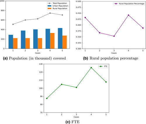
Figure 11b shows the rural population percentage covered by the HPSAs for all the cases. Case 3 has the lowest rural population percentage due to its same parameter setting for rural and urban areas, and also indicates the disadvantages of rural areas in the traditional methods. Case 4 has the highest rural population percentage. In Figure 11c of total Full-Time Equivalent providers covered, Case 4 also obtains the maximum value. Case 5 has the smallest population constraints, but the performance drops for Case 5, with a lower rural population, slightly higher urban population and lower FTE compared with Case 4. Therefore, Case 4 is used as a representative result of our proposed method using the random walk algorithm.
4.5 GIS tools for automating the RSA and HPSA delineations
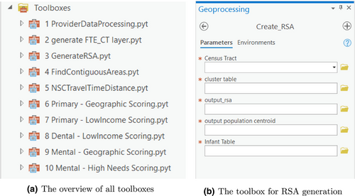
To further support the utilization of the proposed Auto-RSA-HPSA method in public health decision-making, a set of Python toolboxes in ArcGIS is developed. As presented in Figure 12a, this toolbox set has multiple steps including data preparation (tools 1–2), RSA generation (tool 3), candidate HPSAs evaluation (tool 4), travel time calculation (5) and the HPSA scoring steps for all types of HPSAs (tool 6–10). The whole process follows the Shortage Designation Process (HRSA, 2020a) and is developed under iterative discussions with the state officials from the Wisconsin Department of Health Services. The community detection for RSA development is completed in an external Python script that can be executed automatically with different rural/urban parameters. The community/RSA membership result is used as one input for the toolboxes. Figure 12b shows the required parameters for creating RSAs in tool 3. The user needs to provide the base census tract layer from the previous toolbox (step 2), and the community membership file. Then, the toolbox can generate the RSA layer and the population centroid, which can be further used for HPSA scoring.
5 CONCLUSION
RSAs are fundamental units to understanding healthcare markets and evaluating the resource allocation effectiveness. In this research, we propose a travel data-driven and spatially constrained community detection method with the consideration of rural/urban differences to identify RSAs. By doing so, the method can better reflect the fact that health resources are unevenly distributed across space. The proposed method generates more regularly shaped RSAs and is more balanced in region sizes than other baselines. The identified RSAs are further used to establish the Health Professional Shortage Areas (HPSA) through multiple spatial and non-spatial health scoring criteria. The introduction of rural/urban parameters helps identify more shortage areas, cover more rural populations and receive higher shortage scores. The result demonstrates the importance of such consideration by showing more rural shortage areas can benefit from the new designation plan. The method also provides more possibilities for solving such health inequality problems using GIS tools.
The proposed method is a data-driven approach without any additional manual adjustment if using our default parameter settings. Compared with the manual process that many public health officials are using, this method builds a carefully designed methodological framework that can be automated through the provided toolbox. In addition, the result RSAs can be generated at different geographic scales. One can adjust the population constraints based on different regional characteristics to create desirable area sizes. Due to this ability, the method can support repeatable and efficient analysis to assess the results under different scenarios. This also helps policymakers evaluate the proposed RSA plan in a more consistent and statistically sound way. In addition, we have developed the Python toolbox embedded in a GIS environment that requires very little programming knowledge to execute. This enables a broader range of users to access the toolbox and conduct analyses on their own.
Compared with existing studies, which mostly used patient-hospital flows, this study uses openly accessible mobility-based health place visits to extract RSAs. The mobility patterns may provide another dimension to understanding the local healthcare market as it reflects how people travel to receive health services. As shown by the result, there is valuable information from human mobility that can support better RSA and HPSA development in the public health domain.
There are also some directions to improve for future work. First, the spatial network is directed in reality but taken as undirected in this research. More analyses can be conducted to understand the effects of different graph construction methods on the final RSA/HPSA results. Second, the health visits data used in the method may still contain some bias as it may not include all the health-related places; we suggest adding more analyses and comparing with improved Dartmouth methods with hospitalization data when available. Also, the mobility flow is from people's home locations to different places, while people may also travel from work locations to visit providers/hospitals, which can be explored in the future.
ACKNOWLEDGMENTS
We would like to thank the SafeGraph Inc. for providing the data about anonymous location visits and the Wisconsin Department of Health Services Primary Care Program for providing the health resource data and thank Aleksandr Kladnitsky, Regina Vidaver, Penny Black, and Jaime Olson for their guidance on this research.
CONFLICT OF INTEREST STATEMENT
The authors declare no conflict of interest.
Open Research
DATA AVAILABILITY STATEMENT
The Python code used in this research is publicly available on GitHub: https://github.com/GeoDS/Auto-RSA-HPSA. The census track-level mobility flow dataset used is publicly available on GitHub: https://github.com/GeoDS/COVID19USFlows. The geographic boundary data that support the findings of this study are available from the U.S. Census Bureau. Due to the privacy protection policies of the health data providers, the healthcare FTE data used in the research are not publicly available.


