Deep learning approaches for delineating wetlands on historical topographic maps
Abstract
Historical topographic maps are an important source of a visual record of the landscape, showing geographical elements such as terrain, elevation, rivers and water bodies, roads, buildings, and land use and land cover (LULC). Historical maps are scanned to their digital representation, a raster image. To quantify different classes of LULC, it is necessary to transform scanned maps to their vector equivalent. Traditionally, this has been done either manually, or by using (semi)automatic methods of clustering/segmentation. With the advent of deep neural networks, new horizons opened for more effective and accurate processing. This article attempts to use different deep-learning approaches to detect and segment wetlands on historical Topographic Maps 1: 10000 (TM10), created during the 50s and 60s. Due to the specific symbology of wetlands, their processing can be challenging. It deals with two distinct approaches in the deep learning world, semantic segmentation and object detection, represented by the U-Net and Single-Shot Detector (SSD) neural networks, respectively. The suitability, speed, and accuracy of the two approaches in neural networks are analyzed. The results are satisfactory, with the U-Net F1 score reaching 75.7% and the SSD object detection approach presenting an unconventional alternative.
1 INTRODUCTION
Historical maps present a useful depiction of bygone landscapes with diverse types of information. Such information can be used for various purposes such as urban planning, archeology, baseline for change evaluation, and finally, environmental analysis for different purposes, such as nature conservation and restoration. For the last mentioned use-case, analysis of land use and land cover (LULC) changes is critical.
In the case of hydrological assessment and mitigation of climate change impacts on the landscape, the center of attention is water availability in the landscape, and, in this article, particularly wetlands. Wetlands are among the most productive ecosystems and provide valuable ecosystem services, such as water retention and purification, regulating climate, preventing food and erosion events, maintaining high biodiversity, and serving for recreational purposes (Keddy, 2023) They are important for primary production, carbon capture and carbon storage, and are thus important mediators of global warming and climate change (Hesslerová et al., 2019; Were et al., 2019). Protection and restoration of wetlands is thus one of the most important nature conservation priorities, and understanding their history provides a key for designing current and future measures for conserving water resources and increasing resistance of the modern landscape to global change (Beller et al., 2020; Erős et al., 2023).
Despite the significance of this kind of data for understanding the landscape and ecosystem processes, recent efforts have only just begun to automate the digitization and extraction of coherent information from such maps, moving away from manual raster image examination. The Czech Republic has a long tradition of topographic and cadastral mapping, with the first comprehensive map of the territory being the Stable Cadastre (Brůna & Křováková, 2006) and derived Imperial Obligatory Imprints of the Stable Cadastre finished in the first half of 19th century. Other historical maps include State Map 1: 5000 – Derived (SMO-5) from the 1950s, Base Maps (ZM) and Military Topographic Maps (TM) at multiple scales. This long tradition is valued for multitemporal analyses of landscape change.
In order to properly analyze any phenomenon depicted on the map, it needs to be scanned into a raster image (Talich et al., 2011) and subsequently digitized to the vector equivalent. The preferred resolution of the scan with regard to the demands of automatic processing was established at 300 dpi (Oka et al., 2012). After scanning, the digitization can be conducted manually on screen, requiring an operator to recognize and trace the map elements with a cursor. Depending on the demanded outcome, the digitizing task can consist of line/polygon (contour, boundary) vectorization, LULC classification (Pindozzi et al., 2015), symbol detection and localization, text recognition, and others.
This highly laborious approach fueled demand for deployment of (semi)automatic methods for this task. A comprehensive holistic approach to semiautomated map processing was conducted by Schlegel (2023). Examples of somewhat successful automated vectorization attempts include Iosifescu et al. (2016), describing parameter setting for each different map, Oka et al. (2012), segmenting contours based on their HSV values, and Kratochvílová and Cajthaml (2020), leveraging ArcScan to automatically vectorize contours. However, all these studies work with thresholding of pixel values to segment a binary map, to be vectorized later by thinning or fitting a centerline.
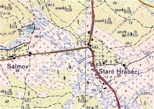
Automated classification of LULC on historical maps can be very simple in case of uniform, color-consistent symbology, such as straightforward Bayesian classification of water bodies (Talich et al., 2018), and the supervised learning toolset HistMapR (Auffret et al., 2017). Due to the peculiar nature of wetland symbology (Figure 1), these simple methods are not capable of segmenting the wetland area coherently and without gaps. Marked with horizontal blue lines, wetland symbols vary in spacing, length, and shade between various samples. With inconsistent symbology and irregular scattering, amplified by the fact that TM10 map sheets were created gradually during a period of nearly two decades, even the manual annotation result can be ambiguous. As the symbology does not consist of a clearly defined boundary, it is often unclear whether two wetland instances are supposed to be merged or separated. As a solution to these problems, we propose to use the deep learning (DL) approach (Minaee et al., 2021).
In the field of geomatics, DL has been utilized with various types of data, most prominently in the realm of remote sensing (Yuan et al., 2020, 2021). Besides other use-cases, such as image registration and change detection, semantic segmentation is widely used to classify and label pixels based not only on their spectral properties, but also taking into account their spatial context (Li et al., 2022). Among the DL algorithms applied on raster data, CNNs (Convolutional Neural Networks) are adopted the most frequently (Li et al., 2022). Some of the neural networks used for such purposes include AlexNet, FCNs (Fully Convolutional networks), SegNet, DeepLab and U-Net (Ronneberger et al., 2015; Yuan et al., 2021). The U-Net neural network was initially developed for biomedical image segmentation, but quickly found its way to other fields of profession. Unlike conventional machine learning, DL techniques can learn spatial context to acquire a better understanding of raster data, potentially at multiple scales.
In the context of historic maps, the volume of published research dealing with DL is notably smaller than in remote sensing or other geomatic areas. Nonetheless, studies have been published. Uhl et al. (2017) used the CNNs (LeNet) to segment human settlements and urban areas from USGS historical TM but with a high percentage of false-positives. Liu et al. (2020) investigated the possibilities of CNN on broad segmentation based on superpixels and watershed transform. This approach achieved success but is completely unsuitable for the wetland segmentation task at hand. Petitpierre focused extensively on segmentation of historical city maps (Petitpierre, 2020) and postulated a robust generic segmentation for many types of maps (Petitpierre et al., 2021). Garcia-Molsosa et al. (2021) utilized U-Net CNN segmentation to preliminarily detect archeologically significant localities. Maxwell, Bester, et al. (2020) used a modified U-Net CNN to segment historic surface mine disturbances and evaluated its ability to generalize. Also, the impact of the training sample size on the resulting performance was assessed. Ståhl and Weimann created a simple neural network for a very similar purpose, extracting wetlands from Swedish TM (Ståhl & Weimann, 2022). Jiao et al. faced a similar problem in Switzerland and trained a successful U-Net network (Jiao et al., 2020).
Aside from the semantic segmentation task, numerous studies made use of object detection frameworks, developed to detect, and label desired elements with a bounding box described by its coordinates. These detectors at first acted iteratively, based on a region proposal algorithm, an example being RCNN (Region-based CNN) (Girshick et al., 2014). However, a more effective approach was recently adopted with the ability to detect the features in one step. Some of these networks include SSD (Single-Shot Detector) (Liu et al., 2016), YOLO (You Only Look Once), and its various versions (Li et al., 2023; Redmon & Farhadi, 2017). Li et al. (2018) explored locating and recognizing text from TM using Faster RCNN networks. Saeedimoghaddam and Stepinski (2019) used the same network to localize road intersections from historical maps and found the algorithm is sensitive to complexity and blurriness of the maps. An implementation of this network is Mask RCNN, extending the framework to perform semantic segmentation within each region using CNNs (He et al., 2017). This was successfully used to segment an elevation slope map derived from LiDAR data to delineate mining-related valleys (Maxwell, Pourmohammadi, & Poyner, 2020).
In this case study, we are comparing two approaches for DL-aided delineation of wetlands on TM10 maps. One of them uses a standard U-Net semantic segmentation, the second one uses SSD network for object detection, merging the outputs into a class map. With successful training, U-Net is a proven standard (Jiao et al., 2020; Maxwell, Bester, et al., 2020; Ståhl & Weimann, 2022) for extraction of LULC classes, whereas the SSD approach is more unconventional.
2 MATERIALS AND METHODS
In this article, we analyze Topographic Maps of the General Staff of the Czechoslovak Army 1: 10000 (TM10 maps), created between 1951 and 1971 for military purposes. These maps were produced using aerial photogrammetry and tachymetry, consisting of seven colors, depicting various LULC elements, and include elevation in the form of contour lines. In total, 6432 map sheets were produced in the Gauss-Krüger, S-52 coordinate system (EPSG 3333 for zone 3), covering the entirety of former Czechoslovakia. After completion, the maps were abandoned by the military and stopped being updated altogether.
The software used for the processing was ArcGIS Pro, version 3.2. Aside from conventional GIS processing toolsets, including raster projection and manual digitization, it also supports numerous DL libraries, such as TensorFlow, PyTorch, cuDNN, and integrates them into its Python API with a convenient user interface. Version 3.2 offers native data augmentation, enabling training of more robust models without the need for Python scripting. Some of the available neural networks include SSD and U-Net, which are the subject of testing.
The site of interest is the National Park of Bohemian Switzerland, Czech Republic (see Figure 2, red). Its area and surroundings were used as testing data, with the ground truth layer being manually delineated with polygons for accuracy assessment. A total of 33 map sheets were set for testing, each of them covering approximately 21 km2. The scanned maps were georeferenced to the known coordinates of the corners of the map sheets using projective transformation, which is deemed to be the best method for this case (Cajthaml, 2011), and a seamless mosaic was created from the processed maps to eliminate parts of maps beyond the frame. The raster mosaic dataset could be used for the process, but ArcGIS Pro often crashes while working such a big mosaic, thus the three mosaics were exported as three big seamless raster images.
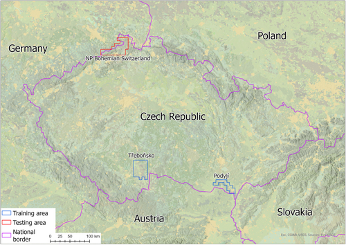
Training data were collected from two other regions, Podyjí and Třeboňsko (Figure 2, blue). Both regions are known for abundant water bodies and wetlands. The wetlands were also manually classified and then exported as image chips of fixed sizes to feed the training process. Sizes of interest are described in Table 1.
| No. of map sheets | Wetland area [km2] | Area [km2] | Pct. of wetlands [%] | |
|---|---|---|---|---|
| Třeboňsko | 32 | 16.9 | 677.2 | 2.5 |
| Podyjí | 15 | 6.7 | 318.9 | 2.1 |
| National Park | 33 | 2.1 | 671.7 | 0.3 |
Both networks require training image chips. SSD works with Pascal Visual Object Classes, exporting an xml file for each chip with the bounding box location, whereas U-Net uses classified tiles as input, adding a classified binary chip of the same location for each single image chip.
2.1 U-Net
The chip size was chosen to be 512 × 512 pixels, representing an area of about 460 × 460 meters. Because we wanted to detect only one type of land cover, no other class was defined. In our case, there are differences in spacing, length, and shade of blue lines between various samples. Because of the variance, a relatively large amount of samples is required and data augmentation is desirable. The wetland symbols are always horizontal, which makes rotating the chips for data augmentation irrelevant except for 180° rotation. Augmentation was also done with striding—chips were overlapped every half of the chip, making the amount of chips roughly doubled in every dimension. Aside from this, brightness, contrast, zoom, and crop were also randomly adjusted to generalize the model and increase its robustness on new data. Overall, 13,168 image chips were exported, all of them included at least a segment of a wetland. Two examples of corresponding image and mask pairs are shown in Figure 3.

2.2 SSD
For neural networks developed for object detection, the choice of the image chip size is usually similar to semantic segmentation, where an object on the chip is marked with a bounding box and fed to the network. Object detection algorithms usually detect an object and mark it with a bounding box. This is very useful when the task is focusing simply on localizing an object on a raster. It is also more suitable for use-cases with dimension invariant objects and generally not a first choice for a precise delineation of boundaries of complex objects, given the geometrical constraints of a rectangular bounding box. This method could be applied to the wetland case as well, but it would result in bad accuracy metrics due to the generalization of potentially complex polygons with rectangles. The wetland symbols are also highly scale-variant, so this approach perhaps would not work at all. For this reason, the size of an image chip was proposed based on the average length of a wetland symbol line, so that the detected rectangles would not generalize much. This resulted in a much smaller image chip size (30 px) and a large amount of image chips. The striding was set at 10 px, resulting in an amount nearing half a million. Image chips fed to this network are depicted in Figure 4.

2.3 Training
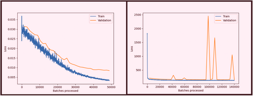
Training was performed with a Nvidia 4070 Ti graphics card processing unit. Validation data percentage was 10% and validation loss was set as the monitoring metric. An early stopping threshold was set for the models not to overfit nor waste unnecessary time for training. Other parameters were set as default. Table 2 describes the model training parameters. Gradual improvements of the models during training can be seen in Figure 5. It is clear that SSD converged rather quickly, whereas U-Net converged more gradually. During SSD training, validation loss sometimes spiked for unknown reasons, but the convergence of training validation is apparent and in the final epoch, validation loss was on its baseline.
| Size of chips [px] | Amount of chips | Training time [hours] | Inference time [hours] | |
|---|---|---|---|---|
| U-Net | 512 | 13,167 | 17 | 0.2 |
| SSD | 30 | 498,020 | 28 | 1.5 |
3 RESULTS
After the training, the model was inferred from test data. The U-Net classification results were converted to polygons without simplification. SSD detections were attached with a confidence attribute, which was thresholded to filter out false-positives. Boundaries of the overlapping SSD detection polygons were then dissolved.
Accuracy metrics were computed based on overlap analysis of polygons. The manually annotated polygons serve as the ground truth. Here also lies the big source of error, because as mentioned in the introduction section, the wetland symbols do not have a clear boundary. Polygons derived from the neural networks inference were not simplified in any way. Summarized areas of these polygons, their intersections, and their ratios were used to describe accuracy.
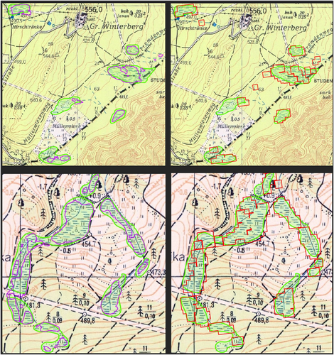
Numerous SSD confidence thresholds were used, and accuracy metrics were calculated in order to find the most accurate result. Also, many false-positives consisted only of one or two detected bounding boxes. This happened because of the limited ability of SSD to take in to account a wider context due to small training chips. Therefore, in addition to the confidence filter, it was decided to remove smaller polygons (under 1000 m2) at the expense of potentially neglecting smaller wetlands. This was applied to all the thresholded datasets with accuracy metrics recalculated. For the sake of experiment, small wetlands were also removed from the U-Net results. The accuracy metrics of the test inferences were calculated and are shown in Table 3. Some examples of segmented wetlands are depicted in Figure 6 along with the ground truth comparison.
| All wetlands | Only wetlands above 1000 | |||||||
|---|---|---|---|---|---|---|---|---|
| Precision [%] | Recall [%] | F1 score [%] | Area [km2] | Precision [%] | Recall [%] | F1 score [%] | Area [km2] | |
| U-Net | 87.9 | 66.4 | 75.7 | 1.59 | 88.6 | 61.0 | 72.2 | 1.45 |
| SSD 90% | 48.4 | 86.9 | 62.2 | 3.78 | 56.8 | 85.1 | 68.1 | 3.15 |
| SSD 93% | 58.7 | 82.1 | 68.5 | 2.94 | 65.0 | 80.0 | 71.7 | 2.59 |
| SSD 94% | 62.7 | 80.0 | 70.3 | 2.69 | 68.3 | 77.5 | 72.6 | 2.39 |
| SSD 95% | 66.6 | 77.1 | 71.4 | 2.44 | 70.9 | 74.2 | 72.5 | 2.20 |
| SSD 96% | 70.3 | 73.7 | 72.0 | 2.21 | 73.8 | 70.7 | 72.2 | 2.02 |
| SSD 97% | 74.7 | 69.7 | 72.1 | 1.97 | 76.3 | 66.0 | 70.8 | 1.82 |
| SSD 98% | 78.8 | 62.2 | 69.5 | 1.66 | 79.8 | 57.3 | 66.7 | 1.51 |
- Note: The last column reports the extent of detected wetlands compared with the manually annotated ground truth layer of 2.10 km2. The results with the best F1 score are highlighted.
4 DISCUSSION AND CONCLUSIONS
This article presented two different approaches for DL-based delineation of wetlands from scanned TM. Two DL models were trained and evaluated independently. Comparing this approach with traditional manual vectorization, DL approach is first and foremost faster and more convenient, especially in the case of larger areas.
On the subject of accuracy, manual vectorization suffers from human errors. In addition, unlike elements with distinct boundaries (buildings or contours), wetland signs cannot be unequivocally vectorized, and they are subject to interpretation of the particular worker. Ståhl and Weimann (2022) previously concluded the greatest error between ground truth and test data comes from disagreement on how the outline borders of the wetlands should be drawn. This phenomenon is amplified in our case, as TM10 wetland boundaries are defined even more vaguely. Furthermore, we mostly deal with small areas, where the bounding parts make up a larger percentage of the total area. Thus, we can expect generally worse statistical metrics of the correspondence of DL detection and ground truth than what would be achieved on map elements with clearly defined boundaries. This factor systematically lowers the perceived accuracy of DL approach since the ground truth is already laden by inherent error.
It is clear from the statistics (Table 3) that the U-Net model is much more conservative in detection than SSD, segmenting overall smaller area, having much higher precision score than recall, seemingly missing many manually delineated wetlands. Figure 6 (left) generally explains this phenomenon, where the model generally segments only the immediate surroundings of the blue lines marking wetlands, whereas the ground truth polygons (manually vectorized) accommodate the broader context of the wetlands. To bring the U-Net results closer to the ground truth, a buffer operation might be applied, but this again triggers the doubt of whether the ground truth dataset is unquestionably faultless.
The SSD, on the other hand, achieved a much higher recall score at the expense of precision, with F1 score being significantly lower than U-Net's. This is partly due to the generalization aspect of the object detection concept, fitting the polygons with rectangular bounding boxes. The SSD, however, showed generally higher recall scores compared with U-Net (better omission error). Precision is lower because of a high number of false-positive detections (example in Figure 6 upper right), where similarly looking elements were mistakenly judged as wetland lines. This applies mostly to watercourses in a horizontal direction and seasonal watercourses marked with dashed lines. These false-positive detections are mostly detected with only one or two adjacent bounding boxes. Also, the rectangular shape of detections does not properly delineate the borders of the wetlands and creates small holes. This would require some kind of generalization operation to bring it up to cartographic standards, such as Douglas-Pecker algorithm.
SSD results were thresholded at various confidence percentage values and all of these versions were also trimmed at 1000 m2 to find the most accurate method. With the best set of parameters, F1 score was comparable with U-Net's, achieving up to 72.6%. The SSD model best performed when capped at 97% confidence. Removing small wetland detections moved the performance equilibrium somewhat lower, toward 94–96% interval. However, this approach generally improved recall at the expense of precision.
The U-Net model was simpler to train, requiring a much smaller amount of training chips, even though they covered the same extent. Also, both the training and inference were faster. However, utilization of the unconventional SSD model brought some interesting results, encouraging its potential development and use for a variety of use-cases. A similar process would work with any other map symbol, likely with better success in the case of scale and rotation invariant symbols. The difference between SSD and U-Net results might be linked to the training chips size, as Petitpierre et al. (2021) pointed out that by removing color and texture, the performance of U-Net segmentation decreases only marginally, as the network focuses on high-level cues. In his research, he used 1000 px chips. We used comparably very small chips for SSD network, which are unable to consider any wider context. This undeniably influenced the outcome.
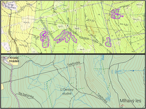
The trained models can be easily applied to all TM10 maps with similar expected results. Old maps are an important source of data in landscape restoration planning to restore the landscape's ability to retain water and useful for the identification of both vanished water bodies and vanished wetlands. Despite the mentioned imprecision, the trained neural networks make the identification of former wetlands within the TM10 maps fast and can be used statewide in landscape restoration efforts to mitigate negative consequences of climate change. Figure 7 shows an example of frequent man-made drainage of wetlands, an intervention now considered harmful to the environment and its diverse ecosystem. In our research, we used this DL methods to identify vanished wetlands and prepare their revitalization within the project “Water in the landscape of Bohemian Switzerland” in the area of the Bohemian Switzerland National Park and the Elbe Sandstone Protected Landscape Area (Müllerová et al., 2023).
ACKNOWLEDGMENTS
This research was funded by Student Grant Competition of Czech Technical University in Prague, grant SGS24/050/OHK1/1T/11 (JV), and by Technology Agency of the Czech Republic, project SS05010090 (all authors). Open access publishing facilitated by Ceske vysoke uceni technicke v Praze, as part of the Wiley - CzechELib agreement.
CONFLICT OF INTEREST STATEMENT
The authors declare no conflict of interest.
Open Research
DATA AVAILABILITY STATEMENT
The data that support the findings of this study are available from ČÚZK. Restrictions apply to the availability of these data, which were used under license for this study. Data are available from the author(s) with the permission of ČÚZK.


