Accounting for length of hospital stay in regression models in clinical epidemiology

1 INTRODUCTION

In performing risk factor analysis of hospital-acquired infections (HAIs), researchers are confronted with the competing risks of discharge or death without HAI (see Wolkewitz, Cooper, Bonten, Barnett, & Schumacher, 2014). Time at risk (TAR) for HAI is the time in hospital without an infection. The risk of acquiring an HAI is dependent on the duration of time a patient is at risk. This time dependency in this kind of setting has been previously discussed, for example, in Akre, Thulin, and Bottai (2013).

It is frequently the case that in observational studies only the length of stay (LOS) is known, whereas the time of infection is not (e.g., Giuliano, Baker, & Quinn, 2018; Kyaw et al., 2015). In this situation, it is not possible to obtain the exact TAR, and hence, it is only possible to work with LOS. There are different approaches to adjust for LOS or TAR in regression models. In the literature, there are several examples of investigating HAI using odds ratios (ORs) adjusted for LOS or TAR in order to model the effect of other risk factors on HAI accounting for either time measure (e.g., Djordjevic, Markovic-Denic, Folic, Igrutinovic, & Jankovic, 2015; Eyre et al., 2018; Wong, Chen, Win, Ng, & Chow, 2016). It is important to distinguish between adjusting for LOS or TAR, as different problems affect the two approaches. One limitation of controlling for LOS is obvious: Because these infections are intermediate events between admission and discharge, the overall length of hospital stay of infected patients is the sum of the time before and the time after infection. For patients with an infection, LOS can only be determined after the occurrence of the infection. It is likely that the infection itself has an impact on LOS. Pierce, Lessler, and Milstone (2015) state that LOS might be affected by both a risk factor and the HAI itself. This example of “conditioning on the future” also affects TAR, to a lesser extend, as TAR can only be determined at the time point when the event of interest or the competing event occurred and not at baseline (admission to the hospital).

However, conditioning on LOS is also problematic in ways that are underappreciated. To our knowledge, the interpretation of logistic regression adjusted for LOS has not yet been investigated. While some articles have compared logistic regression and Cox regression (e.g., Chevret, 2001; de Irala-Estévez et al., 2001; Pierce et al., 2015), only Pierce et al. (2015) consider time adjustment, and states only that this introduces bias and should not be done.

As logistic regression adjusted for LOS is frequently used for risk factor analysis of HAI, we feel the need to take a closer look at what time-adjusted ORs actually represent in this context. In this paper, we consider an illness–death model with HAI as an intermediate event, and discharge or death as the absorbing state. Using this model, we consider appropriate analyses, incorporating competing risks to derive reference measures. These include the cumulative incidence function (CIF), cause-specific hazard ratios (CSHRs), and subdistribution hazard ratios (SHRs). While we focus on these approaches, it should be noted that other approaches have been developed to investigate HAI. For instance, absolute risk regression (Gerds, Scheike, & Andersen, 2012) is a useful tool for investigation of the absolute risk of acquiring an HAI. Note that the term absolute risk corresponds to the cumulative incidence.

In the following sections, we investigate the use of these methods of incorporating LOS in predicting the occurrence of HAI. In Section 2, we presents preliminary considerations, followed by a description of the various methods in Section 3. In Section 4, we discuss logistic regression adjusted for LOS from a mathematical point of view and compare logistic regression adjusted for LOS with the CIF using a real data example. In Section 5, different simulation scenarios are considered to illustrate the potential for biased effect estimates with the use of logistic regression adjusted for LOS. We focus on risk factor analysis incorporating a binary covariate with an effect after the occurrence of HAI. We perform risk factor analysis via logistic regression incorporating LOS as a covariate and HAI as the dependent variable. The resulting time-adjusted ORs are then compared with the true underlying effect.

2 PRELIMINARY CONSIDERATIONS

First, we want to focus on the question: Why isn't it a good idea to include LOS as a covariate in the logistic regression model?

In order to answer this, let us consider the statistical quantity calculated. As described above, the occurrence of HAI is a time-dependent process. The aim of including a time variable in the logistic regression is to model the infection depending on time. However, this is not what is being done. The logistic regression adjusted for LOS considers the following probability:

with Y being the infection indicator and T^∗ representing LOS. Note that logistic regression without time adjustment models the probability of developing an infection during the entire hospital stay. A logistic regression adjusted for LOS models the probability of the occurrence of a previous infection, given the duration of hospital stay. It is actually asking what happened in the past, given the knowledge that a patient had a LOS of a certain time. The approach of predicting the risk of infection depending on LOS is inappropriate, as it conditions on the future (see Andersen & Keiding, 2012).

When investigating HAI, we consider two perspectives with respect to HAI. First, a clinician is primary interested in the factors associated with the risk of HAI for a patient during the entire hospital stay, or in more detail, the clinician is interested in factors associated with the risk of HAI for a patient during the next t days. In contrast, an epidemiologist is primary interested in factors associated with the risk of HAI adjusted for LOS at risk. This translates into factors associated with the daily risk of HAI.

A clinician wants to predict patients' outcome (perspective 1); an epidemiologist wants to explain the etiology (perspective 2; Table 1).

Table 1. Two perspectives for risk factor analysis of hospital-acquired infection (HAI) and the corresponding measure of interest in the illness–death model

Perspective	Medical question	Corresponding	Regression	Regression
		measure	method	coefficient of
				interest ( )
Perspective 1 (clinician):	“What is the cumulative risk of an infection	(The plateau of the CIF)	Logistic	OR
cumulative risk of HAI	during the entire hospital stay?”		regression
	“What is the cumulative risk		Regression	Ratios of the
	of an infection during the next		analysis via	corresponding
	t days?”		ARR, LLR, Fine,	cumulative
			and Gray	incidences, OR,
				SHR
Perspective 2 (epidemiologist):	“What is the daily/instantaneous	λ01	Separate
a etiology of HAI	risk of HAI?”		analysis with
	“What is the daily/instantaneous	λ02	two cause-	CSHR
	risk of the competing event?”		specific hazard
			analysis

• Note. λ_ij is the constant transition hazards from state i to j with i,j∈{0,1,2}. CIF = cumulative incidence function; ARR = absolute risk regression; LLR = logistic link regression; OR = odds ratio; SHR = subdistribution hazard ratio; CSHR = cause-specific hazard ratio.

For both perspectives, there exist appropriate regression models. For perspective 1, the clinicians' perspective, the most simple approach is standard logistic regression. Standard logistic regression addresses the cumulative risk of HAI during the entire hospital stay. While this is a rather crude approach ignoring the time dependency, there are more sophisticated approaches such as absolute risk regression, logistic link regression, and Fine and Gray regression of the subdistribution hazard (see Fine & Gray, 1999; Gerds et al., 2012). These regression models incorporate the time until the infection occurred and address the cumulative risk of HAI during the next t days.

Considering perspective 2, the epidemiologists' perspective, there is cause-specific Cox regression for investigation of the daily risk of HAI and the competing event (see Beyersmann, Allignol, & Schumacher, 2012).

Standard logistic regression adjusted for LOS wants somehow to address both perspectives. For instance, Eyre et al. (2018) considered logistic regression adjusted for LOS in order to detect risk factors while controlling for LOS.

As stated before, investigation via standard logistic regression (without time adjustment) corresponds to perspective 1. The probability of the occurrence of an HAI during the entire hospital stay is modeled. The obtained OR is also a measure on the risk scale and quantifies the likelihood of developing an infection during the hospital stay (Ghilagaber, 1998). However, it is a rather crude measure as it does not incorporate the time dependency.

If time-adjusted ORs are considered, the aim is to account for temporal dynamics. Nevertheless, it remains unclear how the adjustment impacts the results.

In the following section, we introduce the illness–death model as depicted in Figure 1 and refer the considered reference measures for the two perspectives.

3 ILLNESS–DEATH MODEL AND REFERENCE MEASURES

In order to highlight the differences between the two perspectives introduced before, it is informative to examine the illness–death model depicted in Figure 1.

For simplicity, we only consider one combined competing risk, representing discharge or death. As we are interested in infection, this does not impact the results. The TAR for developing an infection is the time from admission until a patient leaves the initial state 0 and either the event of interest (transition to state 1) or the competing event occurs (direct transition from state 0 to state 2). LOS is the time from admission until the patient is discharged or dies (transition into state 2, either passing through the intermediate state or not). For patients experiencing HAI, LOS can be split into preinfection and postinfection time (time before HAI and time after HAI, corresponding to the time in state 0 and time in state 1, respectively). Consider X(t)∈{0,1,2} to be a stochastic process, indicating the state an individual is in at time t. λ_ij(t) denotes the transition hazard from state i to state j at time t and is given by λ_ij(t)dt=P(T_i∈[t,t+dt),X(T_i)=j|X(t)=i) (i,j∈{0,1,2}). T_i represents the time of leaving state i (event time) and dt is the length of a small time interval (compare with notation in competing risks situation in Beyersmann et al., 2012).

For simplicity, we assume constant hazards. In general, it might not be the case that the hazards are constant over time. However, we think that, for the illustrative purpose of this work, the use of constant hazards is appropriate.

Consider again the two perspectives and the illness–death model depicted in Figure 1. Analysis approaches and raised questions for each perspective are listed in Table 1. Perspective 2 can be investigated by performing separate analyses of λ₀₁ and λ₀₂. The regression coefficients of interest ( ) are CSHRs. The cause-specific hazard analysis addresses the daily risk of each event, the event of interest, and the competing event. On the other hand, perspective 1 can be investigated via a joint analysis of λ₀₁ and λ₀₂. The subdistribution hazard analysis investigates the probability of an infection over time and the regression coefficients of interest are SHRs. The SHRs correspond to the effect of a covariate on the subdistribution hazard. The understanding of the subdistribution hazard requires some experience and the interpretation can be challenging to communicate. However, SHRs allow for an interpretation as effects on the cumulative incidence. Austin and Fine (2017) give a nice explanation of the respective estimates.

Note that the corresponding measures with respect to the two perspectives do not depend on λ₁₂ (see Table 1), whereas LOS is affected by each transition hazard of the illness–death model, in particular by λ₁₂.

In the next section, we assume the illness–death model as depicted in Figure 1 to be the correct model. We define it as the reference model as it incorporates competing risks and allows for direct interpretation (see Wolkewitz et al., 2014; Wolkewitz, von Cube, & Schumacher, 2017).

4 CIF AND PREDICTED RISK VIA LOGISTIC REGRESSION FROM A MATHEMATICAL POINT OF VIEW

4.1 Mathematical formulation

Consider the definition of the CIF of HAI and the probability of HAI considered by logistic regression. Note that these are measures of different models with different assumptions. Hence, it is expected that they differ. However, as they are used in the same context, we want to point out the differences. Let λ_ij (i,j∈{0,1,2}) denote the constant transition hazards from state i into state j. Recall that T₀ represents the time of leaving state 0, and with t being the time since admission, the CIF of HAI can be written as

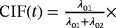
(1)

(see Beyersmann et al., 2012).

According to Gerds et al. (2012), the CIF can be investigated using following transformation model:

(2)

with being a known differentiable function. Considering , formula 2 becomes the logistic link model.

On the other hand, including LOS or TAR as a covariate in a logistic regression with the infection indicator as outcome, the model is as follows:

(3)

with α₀ being the intercept and α₁ being the slope. Recall that T^∗ represents LOS. Given formula 3, the probability of acquiring an infection, conditioning on a given time can be obtained by

(4)

Note that logistic regression assumes a linear relationship.

Comparing the models of formula 2 and formula 3, we observe a difference in the outcome that is considered. With , formula 3 can also be written according to formula 2:

(5)

The logistic link model of formula 2 considers the cumulative incidence up to time t, that is, CIF(t), whereas the logistic regression model of formula 3 considers the overall occurrence of an HAI, that is, 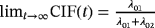corresponding to the plateau of the CIF, and considers the included time variable as a baseline variable.

4.2 Illustration using real data

In order to illustrate the differences between the CIF and the logistic regression model depicted in Section 4.1, we use the SIR3 data from the kmi-package available in R. SIR3 is an observational cohort study. The data contain information on hospital-acquired pneumonia, discharge, and death. In this section, HAI refers to hospital-acquired pneumonia, as this is the infection of interest. Considering HAI as the event of interest, the competing event is discharge or death.

Figure 2 illustrates the overall LOS of an infected patient (left panel). The time of infection divides the LOS into preinfection and postinfection time. For infected patients, LOS is always greater than the actual TAR for acquiring an infection. Thus, when considering LOS as time variable, the corresponding risk set at a specific time point is larger than it is while considering the actual risk set corresponding to the TAR (right panel of Figure 2). Note that, in this data example, the occurrence of the intermediate event is low. If the occurrence increases, the gap between the curves increases, too.

The data set contains information from 1,313 subjects. Of those, 108 (8.23%) developed HAI during the hospital stay, whereas 1,189 (90.56%) were discharged or died without HAI. Censoring was low: 16 subjects were censored without HAI and five subjects were censored after HAI. Logistic regression cannot handle censored observations directly, and it is unknown whether the 16 subjects censored without HAI developed HAI during their hospital stay. Furthermore, for the five subjects censored after the occurrence of HAI, LOS is unknown. Thus, observations of these 21 censored subjects were excluded from both analyses, that is, logistic regression and the multistate approach. Note that estimation of the CIF and CSHRs allows for censored observations. In general, exclusion of censored observations impacts the estimated CIF and is not recommended. However, as censoring is low and thus the estimates should not be affected much, and for the illustrative purpose of this data example, we think that exclusion of the censored observations is justifiable. Data analysis was carried out using R version 3.5.2 with the packages survival and etm.

Logistic regression with HAI as the dependent variable and LOS as the independent variable was performed (intercept=−3.26 [−3.59; −2.95]; slope=0.044 [0.033; 0.055]; OR=1.045 [1.034; 1.057]). For LOS, the slope is positive. This implies that, if patients have a long LOS, the probability that they acquired HAI during their hospital stay increases. This effect is significant. The resulting predictions are presented in Figure 3. For comparison, the CIF is also plotted. Note that depending on the model, the labels of the x- and the y-axes differ. In particular, the settings consider different time variables. The CIF considers time to infection, whereas the logistic regression considers LOS. In the plots according to the logistic regression model, LOS is included continuously as considered in the logistic regression, or weekly as categorical variables.

In Figure 3, the plateau of the CIF approaches the overall occurrence of HAI of approximately 8%. It can also be seen that most cases of HAI occur during the first 20 days. In contrast, as indicated above, the predicted probability of HAI given LOS continuously obtained via logistic regression approaches 1.

In conclusion, the comparison of the approaches substantiates the differences between the two models. The CIF illustrates the temporal development of the cumulative incidence. On the other hand, logistic regression adjusted for LOS with the infection indicator as outcome models the plateau of the CIF while considering LOS as a describing baseline covariate.

5 RISK FACTOR ANALYSIS AND TIME DEPENDENCY

In the presence of competing risks, we distinguish between direct and indirect effects of a covariate. A covariate has a direct effect on the event of interest if it affects its cause-specific hazard (λ₀₁). On the other hand, a covariate has an indirect effect on the event of interest if it affects the cause-specific hazard of the competing event (λ₀₂) and, hence, impacts the TAR for the event of interest. To investigate risk factors, the formulas presented in Section 4.1 can be extended by adding a covariate Z additionally to the time covariate (see Gerds et al., 2012). In the following section, we investigate the question of how time adjustment in logistic regression influences the results of risk factor analysis in the presence of competing risks.

5.2 Illustration via simulated data

As discussed earlier, LOS itself can be influenced by the occurrence of an infection. To investigate adjustment for LOS, data in accordance with the illness–death model depicted in Figure 1 is simulated. We use constant transition hazards (with exponential distribution) and consider a binary covariate as risk factor (Z, binomial with p=0.5). For simplicity, we assume no censoring.

In the following, we present five hypothetical scenarios. The simulation procedure is described in Beyersmann, Latouche, Buchholz, and Schumacher (2009) and Beyersmann et al. (2012). Simulation and analysis of the data were carried out using R version 3.5.2. We compare the estimates across the various scenarios in order to investigate whether logistic regression adjusted for LOS is an appropriate tool for incorporating the time dependency of risk of HAI in presence of competing risks, and whether it helps us to understand the underlying process.

Logistic regression adjusted for LOS

LOS can be divided into the time before infection (i.e., TAR), and the time after infection. Thus, LOS might be affected by the occurrence of an HAI itself. A risk factor analysis for the event of interest should not be affected by differences present only after the event occurred.

To investigate adjustment for LOS, we consider five scenarios. Recall that the data are simulated according to the complete illness–death model depicted in Figure 1, that is, with all three transitions. Scenario 1 is the null model. In this scenario, there is no effect of the covariate on any transition. Similarly, in the subsequent scenarios, there is no effect of the risk factor on the event of interest or on the competing event discharge or death without infection. However, there is an effect on the hazard out of the infection state into discharge or death (λ₁₂), prolonging the time in state 1. This effect increases with each subsequent scenario.

Thus, in each of these five scenarios, there is the same underlying process for the transitions out of state 0. There is no effect of the risk factor on the event of interest, neither directly nor indirectly. However, there are differences in the effects of the risk factor on the LOS after the occurrence of an infection. The effect causes a prolongation of the overall LOS as it prolongs the stay in state 1. For instance, this would be the case if a risk factor leads to a later discharge after the occurrence of HAI.

We simulated 100 data sets with 1,000 observations for each scenario (see Table 2 for an overview of the simulations). In Table 3, the means of the estimates of the crude ORs, and the ORs adjusted for LOS are given. LOS is considered continuous and in weekly categories separately. The first line shows the estimates of Scenario 1. Recall that this is the null model without any effect of the risk factor Z. Both the crude and the adjusted ORs are close to one, and are thus close to the true OR. Consider the subsequent scenarios. As the time in state 1 is prolonged in the presence of the risk factor Z, the adjusted OR decreases. This holds for each scenario and for the continuous and categorical LOS. In Scenario 5, the adjusted OR is reduced to almost half of the crude OR. In this scenario the risk factor has the strongest effect on λ₁₂, and consequently the smallest ratio of the ORs. In summary, as the effect of the risk factor on the discharge or death hazard after infection (λ₁₂) increases, the mean of the ORs adjusted for LOS decreases.

Table 2. Overview of simulation settings

	Scenario	λ01	λ02	λ12
Z=0:	1–5
Z=1:	1
	2
	3
	4
	5

• Note. λ_ij is the transition hazards from state i to j with i,j∈{0,1,2}. Z is a binary risk factor (binomial with p=0.5).

Table 3. Mean over all 100 simulations per scenario with decreasing discharge hazard in the exposed group: ORs with and without adjustment for LOS (for Z=0: )

Scenario			CSHR12	OR	Mean	Mean adjusted
					crude	for LOS
						cont.	weekly
1	for Z=1:		1	1	1.01	1.01	1.01
2				1	1.02	0.86	0.89
3				1	1.05	0.75	0.81
4				1	1.03	0.65	0.72
5				1	1.02	0.56	0.64

• Note. λ_ij is the transition hazards from state i to j. CSHR_ij = cause-specific hazard ratio for direct transition from state i into state j with i,j∈{0,1,2}; LOS = length of stay; OR = odds ratio; adj. = adjusted; cont. = continuous; weekly = [0,7),[7,14),[14,21),[21,28),[28,35),[35,42),≥42)).

Despite the fact that the risk factor actually has no effect on the event of interest, estimates based on adjustment for LOS imply that there is an effect. As seen in Scenario 5, these effects can be substantial.

6 CONCLUSION AND DISCUSSION

In this work, we have considered the consequences of modeling hospital-acquired infections via logistic regression adjusted for LOS. This is common in the literature and it is necessary to look more closely at what is really being estimated. The principal problem with using logistic regression adjusted for LOS to predict HAI is that it conditions on the future, and therefore, the resulting estimates are not interpretable. The problem of conditioning on the future also arises when adjusting for TAR instead of LOS (to a lesser extend). We also considered the advantages of using multistate approaches such as competing risk models and the illness–death model and discussed appropriate measures incorporating competing risks as the reference model.

The multistate approach permits the estimation of CSHRs and SHRs, providing a complete model of the pathways through which risk factors affect the occurrence of the event of interest. We can determine the etiology of the infection as we can detect whether there is a direct or an indirect effect of the exposure. Furthermore, we can also determine the cumulative risk of the occurrence of an infection.

In Sections 2, 3, and 4, we pointed out the differences between the different approaches. The respective models address different questions. While the CIF models the temporal development of the cumulative incidence, logistic regression adjusted for LOS models the plateau of the CIF inappropriately, as LOS is incorporated as a baseline covariate. It is important to be aware of the fact that measures such as the CIF and crude ORs do not depend on λ₁₂ whereas LOS does.

To investigate logistic regression adjusted for LOS for risk factor analysis of HAI, we considered five scenarios in a simulation study in accordance with the illness–death model. In each scenario, there was no effect of the risk factor on the event of interest, neither directly nor indirectly. We found that adjustment for LOS in a logistic regression impacted on the risk factor estimate for HAI and that this impact increased with the effect of the risk factor on the discharge or death hazard. A prolonged stay after the event of interest results in an OR adjusted for LOS smaller than the unadjusted OR. Thus, adjustment for LOS might result in the detection of nonexistent effects.

Additionally, we looked at five scenarios inverse to scenarios one to five (data not shown). These scenarios considered the rather unrealistic situation in which a risk factor increases the discharge and death hazard after infection and thus leads to a shortened stay after the occurrence of an infection (CSHR₁₂= 1, 2, 3, 4, 5, respectively). As expected, the results were in the other direction to Scenarios 1–5. With a shortened stay after the event of interest, the ORs adjusted for LOS were larger than the unadjusted ORs, although the effects were not as large as in the more realistic scenarios with a prolonged hospital stay.

In this paper, we considered logistic regression adjusted for LOS. Furthermore, logistic regression adjusted for TAR should be investigated in more detail. Unlike LOS, TAR is not affected by the infection as it corresponds to the preinfection time. However, it is only determinable at the time of the occurrence of the infection.

The data needed for multistate analyses are not always available. It is frequently the case that the time of infection is unknown and that only LOS and whether an infection occurred are available. Methods to handle interval-censored event times already exist (see, e.g., Touraine, Gerds, & Joly, 2017) and can be applied in the situation we described. However, they are typically applied in different circumstances. Usually, there are different observation periods generating censoring intervals for the transition into the intermediate state. Furthermore, if a patient reaches the absorbing state and was still in the initial state in the last observation period, it is uncertain whether or not they passed through the intermediate state. In the situation we described, however, we know whether or not the event occurred, and only if it occurred is the event time missing. No further restrictions on the censoring interval are given and the boundaries are zero and LOS. In the situation where missing information is highly dependent on the event status, we recommend that knowledge of the specific characteristics of the pattern of the missing data should be used to model the event-time, thus making it possible to perform appropriate and interpretable analyses. However, this is not a trivial task, and further work needs to be done in order to solve this issue.

In addition to HAI, the problem discussed in this paper is also relevant in other contexts. The situation where the observation time can be split into two different time frames can also be observed in other kinds of settings, which face the problem of time dependency as described above. For example, when devices such as catheters or ventilation are used, the observation time could be divided into ventilation time before the event of interest and ventilation time after the event of interest. Furthermore, the situation depicted in Figure 1 is also applicable to the study of cancer. Consider the denotation of the states in Figure 1. Birth would correspond to state 0, cancer to state 1, and death to state 2. Hence, LOS represents age at death. In this situation, ORs adjusted for LOS simply quantify the likelihood of whether a person had cancer knowing their age at death.

In this investigation, we assumed no censoring. However, a further problem with logistic regression is that it cannot handle censored observations. In the presence of censoring, one has to decide whether censored observations are treated as missing, thus losing all the information, or whether censored observations are treated as zero, which assumes that censoring is equivalent to “no event.” On the other hand, investigation via the illness–death model using CSHRs and SHRs allows for the handling of censored observations. This is a further advantage of the multistate approach compared to logistic regression. We emphasize that we only considered standard logistic regression. However, a further approach for investigating HAI in this setting is pooled logistic regression. The results of this approach are comparable to the results of a Cox model; see D'Agostino et al. (1990) and Barnett and Graves (2008). Pooled logistic regression is an extension of simple logistic regression that can incorporate censoring.

In conclusion, appropriate methods involving the use of multistate models should be used to capture the time dependency in time-to-event settings, especially in the presence of competing events. We strongly recommend that logistic regression adjusted for LOS should not be used to investigate HAI, as the resulting risk factor estimates are not interpretable. The model does not contribute to a better understanding of the underlying processes and might even lead to wrong conclusions. Further work is required in order to find ways to deal with unknown infection date.