Analytic posteriors for Pearson's correlation coefficient
Abstract
Pearson's correlation is one of the most common measures of linear dependence. Recently, Bernardo (11th International Workshop on Objective Bayes Methodology, 2015) introduced a flexible class of priors to study this measure in a Bayesian setting. For this large class of priors, we show that the (marginal) posterior for Pearson's correlation coefficient and all of the posterior moments are analytic. Our results are available in the open-source software package JASP.
1 Introduction
Pearson's product–moment correlation coefficient ρ is a measure of the linear dependency between two random variables. Its sampled version, commonly denoted by r, has been well studied by the founders of modern statistics such as Galton, Pearson, and Fisher. Based on geometrical insights, FISHER (1915, 1921) was able to derive the exact sampling distribution of r and established that this sampling distribution converges to a normal distribution as the sample size increases. Fisher's study of the correlation has led to the discovery of variance-stabilizing transformations, sufficiency (FISHER, 1920), and, arguably, the maximum likelihood estimator (FISHER, 1922; STIGLER, 2007). Similar efforts were made in Bayesian statistics, which focus on inferring the unknown ρ from the data that were actually observed. This type of analysis requires the statistician to (i) choose a prior on the parameters, thus, also on ρ, and to (ii) calculate the posterior. Here we derive analytic posteriors for ρ given a large class of priors that include the recommendations of JEFFREYS (1961), LINDLEY (1965), BAYARRI (1981), and, more recently, BERGER and SUN (2008) and BERGER et al. (2015). Jeffreys's work on the correlation coefficient can also be found in the second edition of his book (JEFFREYS, 1961), originally published in 1948; see ROBERT et al. (2009) for a modern re-read of Jeffreys's work. An earlier attempt at a Bayesian analysis of the correlation coefficient can be found in JEFFREYS (1935). Before presenting the results, we first discuss some notations and recall the likelihood for the problem at hand.
2 Notation and result
 and covariance matrix

 and
and
 are the population variances of X1 and X2, and where ρ is
 (1)
(1) , where

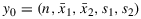
 the sample mean, and
 the average sums of squares. The bivariate normal model implies that the observations y are functionally related to the parameters by the following likelihood function:
 (2)
(2) (3)
(3)
If we set α=β=γ=δ=0 in Equation 3, we retrieve Lindley's reference prior for ρ. LINDLEY (1965, pp. 214–221) established that the posterior of
 is asymptotically normal with mean
 and variance n−1, which relates the Bayesian method of inference for ρ to that of Fisher. In Lindley's (1965, p. 216) derivation, it is explicitly stated that the likelihood with θ0 integrated out cannot be expressed in terms of elementary functions. In his analysis, Lindley approximates the true reduced likelihood hγ,δ with the same ha that Jeffreys used before. BAYARRI (1981) furthermore showed that with the choice γ=δ=0, the marginalization paradox (DAWID et al., 1973) is avoided.
In their overview, BERGER and SUN (2008) showed that for certain a,b with α=b/2−1,β=0,γ=a−2, and δ=b−1, the priors in Equation 3 correspond to a subclass of the generalized Wishart distribution. Furthermore, a right-Haar prior (e.g., SUN AND BERGER, 2007) is retrieved when we set α=β=0,γ=−1,δ=1 in Equation 3. This right-Haar prior then has a posterior that can be constructed through simulations, that is, by simulating from a standard normal distribution and two chi-squared distributions (BERGER AND SUN, 2008, Table 1). This constructive posterior also corresponds to the fiducial distribution for ρ (e.g., FRASER, 1961; HANNIGet al., 2006). Another interesting case is given by α=0,β=1,γ=δ=0, which corresponds to the one-at-a-time reference prior for σ1 and σ2; see also Jeffreys (1961 p. 187).
The analytic posteriors for ρ follow directly from exact knowledge of the reduced likelihood hγ,δ(n,r|ρ), rather than its approximation used in previous work. We give full details, because we did not encounter this derivation in earlier work.
Theorem 1.The reduced likelihood hγ,δ(n,r|ρ) If |r|<1,n>γ+1 , and n>δ+1 , then the likelihood f(y|θ) times the prior Equation 3 with θ0=(μ1,μ2,σ1,σ2) integrated out is a function fγ,δ that factors as
 (4)
(4) (5)
(5) . We refer to the second factor as the reduced likelihood, a function of ρ which is given by a sum of an even function and an odd function, that is, hγ,δ=Aγ,δ+Bγ,δ , where
 (6)
(6) (7)
(7) and where 2F1 denotes Gauss' hypergeometric function.
Proof.To derive fγ,δ(y|ρ), we have to perform three integrals: (i) with respect to
 , (ii)
 , and (iii)
 .
.
- The integral with respect to
 yields
where we abbreviated
yields
where we abbreviated (8)
(8) . The factor pγ,δ(y0) follows directly by setting ρ to zero in Equation 8 and two independent gamma integrals with respect to σ1 and σ2 resulting in Equation 5. These gamma integrals cannot be used when ρ is not zero. For fγ,δ(y|ρ), which is a function of ρ, we use results from special functions theory.
 - For the second integral, we collect only that part of Equation 8 that involves σ1 into a function g, that is,
The assumption n>γ+1 and the substitution

 allow us to solve this integral using Lemma A.1, which we distilled from the Bateman manuscript project (ERDéLYI et al., 1954), with
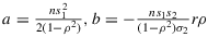 and c=n−γ−1. This yields
where
and c=n−γ−1. This yields
where (9)
(9) (10)and where 1F1 denotes the confluent hypergeometric function. The functions Åγ and B¨γ are the even and odd solutions of Weber's differential equation in the variable
 (11)
(11) , respectively.
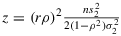
 - With
 , we see that fγ,δ(y|ρ) follows from integrating σ2 out of the following expression:
where
, we see that fγ,δ(y|ρ) follows from integrating σ2 out of the following expression:
where Hence, the last integral with respect to σ2 only involves the functions k and l in Equation 12. The assumption n>δ+1 and the substitution
 (12)
(12) , thus,
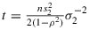
 allow us to solve this integral using Equation (7.621.4) from GRADSHTEYN AND RYZHIK (2007, p. 822) with
 . This yields
After we combine the results, we see that
. This yields
After we combine the results, we see that
 , where
Hence, fγ,δ(y|ρ) is of the asserted form. Note that
, where
Hence, fγ,δ(y|ρ) is of the asserted form. Note that
 is even, while
 is an odd function of ρ.
 is the normalizing constant of the marginal posterior of ρ. More importantly, the fact that the reduced likelihood is the sum of an even function and an odd function allows us to fully characterize the posterior distribution of ρ for the priors Equation 3 in terms of its moments. These moments are easily computed, as the prior πα,β(ρ) itself is symmetric around zero. Furthermore, the prior πα,β(ρ) can be normalized as
 (13)
(13)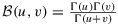 denotes the beta function. The case with β=0 is also known as the (symmetric) stretched beta distribution on (−1,1) and leads to Lindley's reference prior when we ignore the normalization constant, that is,
 , and, subsequently, let
 .
.
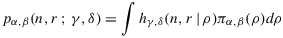
Corollary 1.Characterization of the marginal posteriors of ρ If n>γ+δ−2α+1 , then the main theorem implies that the marginal likelihood with all the parameters integrated out factors as pη(y)=pγ,δ(y0)pα,β(n,r;γ,δ) where
 (14)
(14) (15)
(15) (16)
(16) is the normalization constant of the prior Equation 13, Wγ,δ(n) is the ratios of gamma functions as defined under Equation 7, and
 refers to the Pochhammer symbol for rising factorials. The terms ak,m and bk,m are

Proof.The series E(ρk|n,r) result from term-wise integration of the hypergeometric functions in Aγ,δ and Bγ,δ. The assumption n>γ+δ−2α+1 and the substitution x=ρ2 allow us to solve these integrals using Equation (3.197.8) in GRADSHTEYN AND RYZHIK (2007, p. 317) with their
 and
and
 when k is even, while we use
 when k is odd. A direct application of the ratio test shows that the series converge when |r|<1.
3 Analytic posteriors for the case β=0
For most of the priors discussed earlier, we have β=0, which leads to the following simplification of the posterior.
Corollary 1. (Characterization of the marginal posteriors of ρ, when β=0)If n>γ+δ−2α+1 and |r|<1 , then the marginal posterior for ρ is
 (17)
(17)


Proof.The assumption n>γ+δ−2α+1 and the substitution x=ρ2 allow us to use Equation (7.513.12) in GRADSHTEYN AND RYZHIK (2007, p. 814) with
 and
and
 when k is even, while we use
 when k is odd. The normalizing constant of the posterior pα(n,r;γ,δ) is a special case with k=0.

 .
.Lastly, for those who wish to sample from the posterior distribution, we suggest the use of an independence-chain Metropolis algorithm (TIERNEY, 1994) using Lindley's normal approximation of the posterior of
 as the proposal. This method could be used when Pearson's correlation is embedded within a hierarchical model, as the posterior for ρ will then be a full conditional distribution within a Gibbs sampler. For α=1,β=γ=δ=0,n=10 observations and r=0.6, the acceptance rate of the independence-chain Metropolis algorithm was already well above 75%, suggesting a fast convergence of the Markov chain. For n larger, the acceptance rate further increases. The R code for the independence-chain Metropolis algorithm can be found on the first author's home page. In addition, this analysis is also implemented in the open-source software package JASP (https://jasp-stats.org/).
Acknowledgements
This work was supported by the starting grant ‘Bayes or Bust’ awarded by the European Research Council (grant number 283876). The authors thank Christian Robert, Fabian Dablander, Tom Koornwinder, and an anonymous reviewer for helpful comments that improved an earlier version of this manuscript.
Appendix A: A Lemma distilled from the Bateman project
Lemma A.1.For a,c>0, the following equality holds:
 (A.1)
(A.1) (A.2)
(A.2) , respectively.
Proof.By ERDéLYIet al. (1954, p 313, Equation (13)), we note that
 (A.3)
(A.3)
References
- † We thank an anonymous reviewer for clarifying how Jeffreys derived this approximation.