Optimal Mission Abort Policy for Systems Operating in a Random Environment

1. INTRODUCTION

Most existing system reliability models mainly deal with assessing the probability of performing a required function by a system under the given operational conditions and for a specified period of time.1 Another conventional index is the mission success probability, i.e., the probability of completing a specific mission with or without a deadline.2 However, in practice, there often exist situations when survival of a system, due to safety or cost-related reasons, may have a higher priority than accomplishing the defined mission. In these cases, a mission abort policy can be implemented in order to improve the system survivability and thus to decrease the risk of casualties and/or of substantial economic losses.

A mission is usually aborted when a certain malfunction or incident condition (e.g., external impacts) is satisfied and a safe rescue or recovery procedure is initiated.3 A real-world example of the described scenario is an aircraft that can be required to abort a mission after a certain number of external impacts associated with malicious activity or nature conditions (e.g., lightning inducing electrical peaks in the electrical circuits). These impacts can cause deterioration of critical systems that makes the risk associated with the mission continuation unacceptable.

Traditional system reliability models typically cannot address a possibility of mission aborts while evaluating and optimizing reliability characteristics of engineering systems. In this article, we make a novel contribution by modeling and evaluating the mission success probability and survivability of systems operating in a random environment and subject to mission aborts. An impact of environment is modeled by an external shock process. In our model, shocks affect the system failure rate directly, increasing it a constant amount with each event. We consider a policy when a mission is aborted and a rescue procedure is activated immediately after the mth shock.

Reliability analysis of systems with mission abort policies is a rather new and practically important topic addressed only in a couple of papers so far. In the pioneering paper by Myers,4 the author considered standby systems with an abort policy and a rescue procedure to be initiated upon the failure of a fixed number of components. The corresponding method was developed only for homogeneous, hot standby systems with identical components and exponential time-to-failure distributions. In Levitin et al.,5 the model was extended to heterogeneous systems and the adaptive abort policy. However, these papers do not take into consideration the influence of a stochastic environment on operational characteristics of systems and the corresponding abort policy. Neglecting the effect of a random environment and considering only static models can lead to substantial discrepancies in assessing reliability and safety characteristics of various engineering systems.

There is an extensive literature on shocks modeling in reliability and risk analysis (see, e.g., the following monographs: Nakagawa,6 Finkelstein,7 Finkelstein and Cha8). Traditionally, one distinguishes between two major types of shock models: the cumulative shock models when systems fail due to some cumulative effect and the extreme shock models when systems can fail with certain probabilities upon any shock (Klefsjo,9 Mallor and Omey,10 Gut and Husler,11 Cha and Finkelstein,12 to name a few). In this article, we consider a practically important model when shocks effect the failure rate directly (Cha and Mi,13 Lemoine and Wenocur).14, 15 To the best of our knowledge, there are only a few papers in the literature that consider the number of shocks experienced by a system as a decision parameter for some optimization problems (see, e.g., Finkelstein and Gertsbakh).16 Our challenge in this article is to perform the corresponding analysis for systems with a possibility of a mission abort.

The rest of the article is organized as follows. Section 2. presents the problem formulation. Section 3. defines the corresponding failure model. In Section 4., we derive the mission success probability and the system survivability. Section 5. presents an illustrative example and the corresponding analysis. Section 6 concludes the article and outlines possible directions for future research.

2. PROBLEM FORMULATION

Consider a system that performs a mission task that requires continuous operation during the time τ. Thus, for the mission completion, a system should be operable in [0, τ). Let the lifetime of a system in a baseline environment be described by the cdf with the corresponding failure rate . However, during a mission, a system can be exposed to shocks of different nature that decrease its lifetime and, consequently, the mission success probability as well. In this article, we assume that shocks occur in accordance with the nonhomogeneous Poisson process (NHPP) }, with rate , where is a random number of shocks in [0,t) and are the corresponding (random) shock arrival times. In the model to be described, shocks affect the failure rate of a system directly, increasing it and, therefore, reducing the lifetime.

As was mentioned above, there often exist situations in practice when survival of a system, due to safety or cost-related reasons, may have a higher priority than accomplishing the defined mission. This is obviously the case for safety critical technological processes, experiments, aircrafts, manned space missions, and submarines. In these cases, a mission abort policy can be implemented to improve its survivability. Thus, when the successful mission completion becomes unlikely, a mission should be aborted and a rescue procedure that requires less time than the remaining mission time should be implemented. When damage from shocks is cumulative, and shocks are observable, it is reasonable to consider a number of shocks experienced by a system as the corresponding decision variable. Thus a mission should be aborted upon experiencing m shocks, and the problem is to define this number in an optimal way.

We will first describe the relevant issues regarding the mission abortion and completion and then will address the suggested survival model. It is natural to assume that the time of the rescue procedure is a function of the occurrence time of the mth shock, i.e., φ = φ(t_m), where is the realization of the random (see an example of the nonmonotonic function φ(t_m) in Section 5.). When increases, the remaining mission completion time decreases and eventually, φ(t_m) becomes larger than . Thus, it becomes unreasonable to start the rescue procedure if it takes more time than the remaining mission time. Therefore, we assume that the system continues executing the mission if φ(t_m)≥τ-t_m. Note that we assume also that during the mission time and the rescue stage the same lifetime model holds, which means that the rate of the NHPP of shocks is the same function of time during the primary mission and the rescue procedures. The scenario when, for instance, this rate for the rescue phase is smaller than that for the mission phase can be also of interest and we plan to consider this case in future research.

Let the random variable L denote the system lifetime and ξ (ξ<τ) be the time after which the mission completion takes less time than the rescue procedure, i.e.,

(1)

The value of ξ can be obtained for each specific setting (see the example in Section 5.).

The mission succeeds if the system does not fail in [0, τ) and less than m shocks occur in this interval of time (no mission abort). Notice that in accordance with this definition, the mission still can succeed if , as it is not aborted in this case. In accordance with the above, the mission success probability is R(τ,ξ,m) = Pr(L>τ,T_m≥ξ).

The system survives if it completes either the mission or the rescue procedure. The rescue procedure is activated only if t_m<ξ. To complete the rescue procedure activated at a random time T_m, the system lifetime must be not less than T_m+φ(T_m). Thus, the system survivability is:

(2)

When the decision parameter m is increasing, is increasing in the sense of the usual stochastic order (Shaked and Shantikumar,17 Finkelstein)7 and, therefore, the mission success probability R(τ,ξ,m) is increasing (because the abort probability is decreasing), whereas the system survivability S(τ,ξ) is decreasing. Specifically, when m = 0 (), the system does not perform the mission task and only executes the rescue procedure, which results in R(τ,ξ,0) = 0 and S(τ,ξ,0) = Pr(L>φ(0)). On the other hand, for m = ∞, the system never performs the rescue procedure and survives only if the mission is successfully completed, which gives: R(τ,ξ,∞) = S(τ,ξ,∞) = Pr(L>τ).

The problem is to achieve the balance (tradeoff) between R(τ,ξ,m) and S(τ,ξ,m). For example, the problem of obtaining the optimal m(τ,ξ) that achieves the maximum mission success probability subject to providing a desired level of system survivability S* can be considered, i.e.,

(3)

When the mission failure and the loss of a system are associated with the corresponding costs C_F and C_L, the cost minimization problem with respect to the decision parameter m can be also considered. The probability of a system loss is 1 − S(τ,ξ,m). In this case, the mission also fails and the total cost of losses is C_F + C_L. The probability that the system survives, but the mission fails is (S(τ,ξ,m) − R(τ,ξ,m)). In this case, the total cost of losses is C_F. Thus, the expected cost of losses to be minimized is:

(4)

3. FAILURE MODEL

The proportional or additive hazards approaches for modeling an impact of the continuously changing environment are well established in statistical literature, whereas for the discrete setting, the corresponding modeling is often performed within the framework of the shot-noise processes (see, e.g., Lemoine and Wenocur).15 Therefore, for the lifetime L of a system operating in a random environment described by the NHPP process of shocks , we define the corresponding random failure rate (failure rate process) in a specific, but meaningful form (Cha and Mi,13 Cha and Finkelstein18) that describes an impact of shocks directly on the failure rate of a system, i.e.,

(5)

where is the baseline failure rate of a system (in a static environment without shocks) and is the deterministic jump on each shock. Thus, the effect of each shock is manifested through a jump in the corresponding failure rate, which is a stochastic process now, whereas Equation 5 describes a cumulative-type shock model (Cha and Mi).13 We can observe a part of this process (namely, the number of shocks, m) and can control it. Thus, when a realization of the random failure rate is too large, which corresponds to the sufficiently large m, the mission should be aborted.

The functions and v(t) are usually directly available from statistical data. The practical evaluation of the unobservable parameter η can be based on the failure data analysis. It follows from Cha and Mi13 that, e.g., for the specific case with a constant rate of a shock process, the failure rate of a system operating in the described random environment can be obtained as:

(6)

where expectation is obtained with respect to the process and conditionally on survival in [0, t). Thus, when the baseline failure rate is known, an unobservable parameter η can be estimated from the test failure data with a controlled rate v.

4. MISSION SUCCESS PROBABILITY AND SYSTEM SURVIVABILITY

Recall that L denotes the lifetime of a system that is described by the lifetime model.5 The proof of the following supplementary result can be found in Cha and Finkelstein.18

Proposition 1.The joint distribution of is given by:

(7)

It immediately follows from Equation 6 that:

(8)

4.1. Probability of the Successful Completion of the Rescue Procedure

In accordance with our setting, a general expression for this probability is:

(9)

where denotes the lifetime of a system after the mth shock that occurred at time x (see later), whereas the probability that a system starts the rescue procedure in the time interval [x,x+dx) takes the form:

(10)

where by we mean .

Relation Equation 10 obviously follows from the general properties of the NHPP. From Equation 7, we get:

(11)

Thus, the first multiplier in the integrand in Equation 9 is defined. To obtain the second one, i.e., , we take into account that if the rescue procedure is activated at time x from the start of the mission, then the rate of the shifted NHPP of shocks at time t after activation (to be denoted as ) is and the corresponding random failure rate that describes the lifetime of a system is (compare with Equation 5):

(12)

since exactly m shocks had occurred before the mission abort. Thus using Equation 8, we obtain:

(13)

4.2. Mission Success Probability

Similar considerations hold for obtaining the mission success probability:

Indeed,

(14)

where the first and the second terms in the r.h.s. define the probabilities of completing the mission when there are less than m shock in [0, τ), and when the mth shock had occurred in , respectively. Similar to Equation 9, denotes the lifetime, when the “initial conditions” for the system are given by and defined in Equation 12. Using Equation 7, can be obtained as:

(15)

Finally, using the obtained results, we get the following relationships for and :

(16)

(17)

Consider now a specific case of the homogeneous Poisson process when v(t)≡v and assume that the baseline failure rate is constant, i.e., λ₀(t)≡λ. Then the above equations take the form:

(18)

(19)

5. ILLUSTRATIVE EXAMPLE

Consider an example of an unmanned aerial vehicle (UAV) that should fly from location a to location d performing a surveillance mission (Fig. 1). The distance between the locations that should be covered by the UAV to fulfill the mission is 1,250 km. The UAV speed is 212.5 km/h. Thus the mission time is τ = 1250/212.5 = 5.88 h. There are two safe landing fields b and c that can be used for emergency landing along the route. The locations of these fields are shown in Fig. 1. 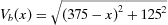If the flight mission is aborted when the distance covered from the airport a is x, the UAV has to cover the distances, , , and to reach locations a, b, c, and d, respectively. The distance to the closest location for the emergency landing is defined by . Fig. 2 shows as functions of the distance covered by the UAV, x when the decision about the mission abort is made. It can be seen that for x>1062.5, and the destination location becomes the closest one. Thus, if the mth shock occurs when x>1062.5, the rescue procedure presumes the mission completion. The distance x = 1062.5 corresponds to the flight time ξ = 1062.5/212.5 = 5 hours. Having and the UAV speed, one can obtain the function defined in Equation 1.

The baseline failure rate that corresponds to the UAV's lifetime is assumed to be a constant (λ). The UAV is exposed to the external shocks caused by lightning with the constant rate v. These shocks affect the failure rate in accordance with Equation 5.

For analysis of the mission success probability R and the corresponding survivability S, Fig. 3 presents these variables as the functions of the decision parameter m and the shock impact factor η for λ = 0.001 and v = 0.2 (assuming v(t)≡v and λ₀(t)≡λ). For convenience of notation in this example, we omit the corresponding arguments, where appropriate.

Figs. 4 and 5 present the solutions of the optimization problem with respect to m: max R(m) s.t. S(m)>0.9 as functions of parameters λ, v, and η. It can be seen that for small failure and shock rates, the UAV survivability remains above the level of 0.9 even without aborting the mission, which corresponds to the optimal value m = ∞, for which R = S.

With increase in shocks impact factor η and in rates λ and v, the mission abort becomes necessary for providing the desired UAV survivability and the optimal number of shocks for the mission to be aborted decreases. On the other hand, starting from certain levels of η, λ and v, the rescue procedure (even if activated after the first shock), cannot provide the UAV survivability above 0.9 (see Fig. 5).

Fig. 6 presents the solutions of the cost minimization problem with respect to m: min C(m) = C_F(1 − R(m))+C_L(1 − S(m)) for C_F = 1, η = 0.03, and v = 0.1 as functions of parameters C_L and λ. It can be seen that with the increase of the cost of the UAV loss C_L, the optimal value of m decreases, which makes the mission abort more likely. The decrease of m causes the increase in survivability S (at the cost of decreasing R).

6. CONCLUSIONS

This article presents a model for obtaining relevant operational characteristics of a failure prone system that is performing a mission. A system is operating in a random environment modeled by an external shock process affecting its time-to-failure distribution. Each shock results in a constant increment in the failure rate, which is described by the corresponding failure model.

If the mission completion becomes problematic, the mission can be aborted and a rescue procedure is activated. Assuming that the decision about the mission abort is made upon occurrence of the mth shock, we present an original method of evaluating the corresponding mission success probability and the system survivability. Based on the obtained results, one can find the value of optimal m that balances the tradeoff between the mission success probability and the system survivability. We illustrate our findings and approach by considering an example of the unmanned aerial vehicle that should fly from one location to another performing a surveillance mission.

We believe that the considered mission abort model can be applied to different fields ranging from space exploration19, 20 to mining21 and other areas. For instance, to save the extremely expensive drilling equipment, the drilling mission can be aborted at some stages. Our approach can also be hopefully applied in healthcare to make the decisions about urgent treatment withdrawal in the case of shocks. For example, when a biotherapy is used for inflammatory bowel disease treatment, infections (shocks) during the treatment (mission) can cause adverse effect. In this case, the decision about the urgent treatment aborting and applying anti-infection measures can be made based on the comparison between the risk of loss of the therapy effect and the risk of the adverse effect of infections.22 Similar considerations can be applied in more general settings while planning treatments of patients with chronic diseases, as these treatments should be aborted (depending on the comparison of the corresponding risks) in the presence of, e.g., some opportunistic diseases. However, definitely, this topic needs further investigation with the help of the health-care professional.

Further research in this direction can employ other models of shock impact on a system time-to-failure (e.g., considering extreme shock models dependent on the previous shocks history). Scenarios when environment for the mission execution and the rescue procedure are modeled by the shock processes with different rates should be also studied. The combined shock model can also be considered when each shock with a given probability results in a failure, whereas with the complementary probability it increases the failure rate by a constant or random amount.