Prior knowledge-infused neural network for efficient performance assessment of structures through few-shot incremental learning
Abstract
Structural seismic safety assessment is a critical task in maintaining the resilience of existing civil and infrastructures. This task commonly requires accurate predictions of structural responses under stochastic intensive ground accelerations via time-costly numerical simulations. While numerous studies have attempted to use machine learning (ML) techniques as surrogate models to alleviate this computing burden, a large number of numerical simulations are still required for training ML models. Therefore, this study proposes a prior knowledge-infused neural network (PKNN) for achieving efficient structural seismic response predictions and seismic safety assessment at a low computation cost. In this approach, first, the prior knowledge inherently within a theoretical dynamic model of a structure is infused into a neural network. Then, by utilizing the few-shot incremental learning technique, this network would be further fine-tuned by only a few numerical simulations. The resulting PKNN would be able to accurately predict the seismic response of a structure and facilitate seismic safety assessment. In this study, the PKNN's accuracy and computational efficiency are validated on a typical frame structure. The results revealed that the proposed PKNN could be used for accurately predicting the structural seismic responses and assessing the structural safety under a low computational cost.
1 INTRODUCTION
Earthquakes as one of the natural disasters may lead to large losses to communities, some of which have effects lasting decades. A critical capability in achieving resilience against this natural hazard is a regional-scale assessment of the seismic safety of large asset inventories (buildings, bridges, wind turbine, etc.) (Javadinasab Hormozabad et al., 2021; Pezeshki, Adeli, et al., 2023). Given the uncertainties associated with both the seismic hazard and the inventory itself, the most fruitful approaches in this area are probabilistic, which inherently require many samplings of structural behavior under many probably ground accelerations. The well-known performance-based earthquake engineering (PBEE) approaches currently lead the way in this arena (Heresi & Miranda, 2023). Within the overall PBEE framework, structural response characterization is a critical task and has drawn many researchers' attention globally (Noureldin et al., 2023; Peña et al., 2010; Priestley, 1997).
The core task of the seismic assessment is figuring out the structural response characteristics under an adequately large suite of probable ground accelerations that exhibit a range of shaking intensities. This is typically carried out through nonlinear time history analyses (NLTHAs) carried out on finite element models of varying sophistication/complexity, wherein uncertainties in modeling parameters as well as ground accelerations are considered (Casotto et al., 2015; Jalayer et al., 2015). Given the compounding uncertainties, the computational costs are usually high, and thus, the regional-scale assessment tasks are typically formidable. For subsequent tasks, such as fragility analysis and resilience-based structural design optimization, this drawback is further magnified. Naturally, reducing the required number of NLTHAs without sacrificing the accuracy of seismic response predictions has become a focal research topic (Jayaram & Baker, 2010).
To increase efficiency, Zhuang et al. (2022) proposed an “enhanced cloud” approach. In the classic cloud method, only peak seismic responses from NLTHAs are used in constructing the probabilistic seismic demand model (PSDM). In comparison, in the enhanced cloud method, the structural responses with corresponding earthquake intensity measures (IMs) within the intensifying excitation range of a ground acceleration from NLTHAs are utilized. Accordingly, the required number of NLTHA is reduced. Similarly, the idea of the “endurance time method,” which also uses intensifying ground accelerations to trigger structural responses from elastic into plastic regimes, has also been used in seismic assessment (Estekanchi et al., 2020). However, it was observed that this approach usually leads to remarkable biases in results, requiring corrections (Basim & Estekanchi, 2015; Pang & Wang, 2021b).
While the aforementioned approaches attempt to reduce the number of NLTHAs with a sophisticated model, another track of work focused on reducing the order of the models themselves through “surrogate” modeling. de Felice and Giannini (2010) opted for a polynomial-type response surface method (RSM) in conjunction with central composite design to directly model the relationships between structural parameters and seismic motion variables and the corresponding maximum structural responses. The accuracy of RSM heavily depended on the number of available numerical simulation samples. The numbers of required response samples for establishing an RSM were observed to grow exponentially with increasing numbers of input variables/parameters. Subsequent studies attempted to lessen the sample burden (Park & Towashiraporn, 2014; Seo & Linzell, 2013).
Recent advances in machine learning (ML) techniques spurred further advances in this area (Yang et al., 2023; Zhong et al., 2023). ML-based methods often take the form of an RSM substitution for establishing a surrogate model (Feng & Wu, 2022; Luo & Paal, 2019). For facilitating structural seismic safety assessment, Panakkat and Adeli (2009) succeeded in approximately predicting the time of occurrence and location of the potential earthquakes based on recurrent neural networks and several seismic indicators. Then, Adeli and Panakkat (2009) further established a probabilistic neural network for predicting the largest potential earthquake's magnitude within a seismic region in the future. Within the specific research track on seismic response prediction and assessment, Ghosh et al. (2018) tried using a support vector regression–based meta-model to improve the estimation of structural seismic reliability. Perez-Ramirez et al. (2019) succeeded in efficiently predicting structural seismic response time history based on a recurrent neural network. Kazemi and Jankowski (2023) achieved predicting seismic limit-state capacities of steel frames with supervised regression ML algorithms. Noureldin et al. (2023) established an explainable neural network for probabilistic prediction of structure seismic response based on a huge NLTHA-generated database. Although these ML-based surrogate models could effectively facilitate the process of seismic assessment, the training of a good ML model also needs plenty of samples coming from the real world or the numerical simulation. Mostly, the sample amount for training an ML-based surrogate model should be at least larger than 10 times the input feature dimension (Zhou, 2021). If the training sample is not ample, the trained ML model would easily gotten into overfitting (Chen & Feng, 2022). Therefore, even with the help of ML, the computational cost of seismic assessment is still high. To solve this issue, Luo and Paal (2023) proposed a novel estimator for efficient structural dynamic response computation for multi-degree of freedom (MDOF) systems based on ML without any training data, but this method has not been validated on more complex structures.
To alleviate the demands for a large training database, the incorporation of domain-specific knowledge into ML models becomes a prevailing trend in the field of ML (Chen & Zhang, 2022), which is represented by the knowledge-based artificial intelligence (KBAI) and physics-informed neural networks (PINNs). KBAI or knowledge-based system (KBS) is mainly based on understanding a comprehensive knowledge base, which is a big repository of unstructured existing knowledge data such as human experience, theory, and previous cases to reason suggestions for solving specific problems (Chen & Geyer, 2023). KBAI has been used in engineering applications as diverse as product design, and industrial equipment fault diagnosis (Sakaguchi & Matsumoto, 1983; Sapuan, 2001). Yang et al. (2014) collected previous shipbuilding experience and design standards, and specifications as a candidate library to facilitate the optimization of a watertight bulkhead in a ship. Li et al. (2020) established a knowledge-based neural network for protecting the power transformer by letting a neural network learn plenty of cases judged by power experts. It can be seen that a KBAI can effectively utilize existing knowledge, a KBAI usually requires a large amount of accurate knowledge data for a knowledge base. Meanwhile, the reliability of a KBAI is determined by the quality of knowledge data. If the knowledge inherently is biased, it cannot be used in KBAI.
As for PINNs, Raissi et al. (2017) first introduced the PINNs in order to use a neural network to infer solutions of ordinary or partial differential equations (ODEs or PDEs). As a result, a PINN could be a surrogate model for the system described by the solved ODEs and PDEs. PINNs were proven to be able to effectively boost learning and reduce data needs in supervised learning issues (Lu et al., 2021a) and have succeeded in solving various problematic issues within mechanics and engineering (Cai et al., 2021). Chen et al. (2022) utilized PINNs along with knowledge-based engineering for estimating the maximum takeoff weight of hypersonic vehicles. Recently, Hu et al. (2024) have succeeded in predicting time histories of the structural seismic responses by PINNs. It is only validated on a simple linear elastic structure because there is no explicit ODE or PDE to describe the nonlinear behavior of a complex structure, and PINNs normally require that the existing knowledge is accurate and can be described in the form of equations, which are then introduced as constraints (or penalties) to the ML algorithm's loss functions. If the knowledge cannot be expressed in explicit ODEs or PDEs, it cannot be directly embedded into PINNs. When the knowledge in ODEs or PDEs is not precise, its inherent error would also be embedded into PINNs. For specific domains such as structural seismic response prediction and assessment, there is not any accurate existing knowledge but only some prior knowledge, which technically cannot be utilized either in KBAI or PINNs (de la Mata et al., 2023).
Against this backdrop, inspired by the idea of KBAI and PINNs about adding knowledge in ML models (Chen et al., 2023; Karniadakis et al., 2021), a prior knowledge-infused neural network (PKNN) model is proposed in this study for achieving real efficient seismic response prediction with low computation cost for training ML. It can also be implemented in seismic assessment. The neural network as one of the prominent ML algorithms, was proved to be capable of approximating any functions (Higgins, 2021). Unlike PINNs needing an explicit PDE to be the loss function (Lu et al., 2021b), in our approach, first, the prior knowledge within a theoretical simplified dynamic model of a structure is embedded into a neural network model in a pretraining stage. Then, the pretrained network model would be fine-tuned by feeding only a few NLTHA samples in an incremental learning process in order to predict the structural seismic response. Through this approach, the number of needed simulation samples could be reduced dramatically while the physical knowledge is utilized to avoid the overfitting issue. It is revealed that the proposed method exhibits both high accuracy and efficiency through a case study of seismic assessing reinforced concrete frames (RCFs). The critical parameters that may impact the effectiveness of the proposed approach are also investigated.
The paper is organized as follows: Section 2 introduces the proposed PKNN for seismic response prediction of structures. Section 3 illustrates how to implement PKNN for seismic performance assessment. Then, in Section 4, the detail of the validation case study is presented, and the relevant results are discussed in Section 5. Conclusions are drawn in Section 6.
2 PKNN FOR SEISMIC RESPONSE PREDICTION OF STRUCTURES
In this section, the workflow and relevant details of the proposed PKNN are explained.
In recent times, artificial neural networks have emerged as one of the most widely utilized ML algorithms. A basic neural network consists of an input layer, an output layer, and several hidden layers, as depicted in Figure 1. In this study, aimed at predicting the seismic response of a structure, the input of a neural network would be the structural and seismic attributes that would influence the seismic response, such as material strength and peak ground acceleration (PGA) of the earthquake, while the output would be the demanded structural response such as maximum interstory drift ratio (MIDR). Each layer within a neural network usually contains multiple neurons. These neurons are interconnected through learned weights and activation functions, such as the “Sigmoid” function. With this structure and adequate training data, as proven by the universal approximation theorem, a neural network possesses the capability to approximate any unknown function (Nishijima, 2021). However, it should be noted that when the training data are limited, a neural network could easily overfit the data. To mitigate this problem, the incorporation of prior knowledge can be beneficial (Raissi et al., 2019). In light of this, the conception of PKNN is introduced, as illustrated in Figure 1.
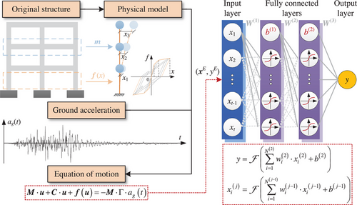
The novelty of using PKNN for seismic response prediction is a specialized two-stage training strategy, including (1) PKNN pretraining and (2) incremental learning on few-shot, as shown in Algorithm 1 where represents the loss function, such as mean square error (MSE). The input of the neural network is designed as a multidimensional feature including structural and seismic parameters, while the output is the demanded structural response. represent the learning weights and hyperparameters for a neural network .
A detailed introduction to these two stages is provided in the following two subsections.
ALGORITHM 1. Pseudo-code of establishing a prior knowledge-infused neural network for seismic response prediction
2.1 Prior knowledge-infused neural network
For the original structure, the physical model shown in Figure 1 and Equation (1) are theoretical and simplified. As a result, the solution of Equation (1) would inherently contain a deviation from the actual response of the structure under the ground acceleration . The structural and seismic parameters and corresponding data are incapable of training a surrogate model to predict accurate structural seismic response. However, is still a reasonable prior estimation of actual structural response and could be useful for pretraining a neural network and making it get close to the demanded accurate mapping relationship between and corresponding structural response. This is like finding a suitable initial point that would be beneficial for an optimization task.
Accordingly, as shown in Algorithm 1, in stage 1, the physical model represented by the equation of motion would be used to generate cheap samples , for initially training the neural network's weights . Superscript “E” of represents these samples are generated by the equation of motion of the physical model. As illustrated above, solving is cost-less in comparison with NLTHA of a refined finite element model, though obtained cannot be used to establish a neural network–based surrogate model for predicting accurate structural responses corresponding to given structural, seismic attributes. Instead, the neural network would initially establish a less accurate relationship between them. The main purpose of this step is to initialize the network and make it closer to the authentic function for predicting structural responses. This process is similar to finding a good initial point of the learning weights and hyperparameters for optimizing the network instead of random start. The obtained neural network is defined as PKNN (Figure 1).
2.2 Incremental learning on few-shot
Then, in the second stage, a small number of the numerical simulation samples would be used for fine-tuning the pretrained PKNN via incremental learning. At this time, with the help of the prior knowledge infused in the first stage, the overfitting issue could be alleviated even though the training data are small. In this stage, one critical point is about how to learn new knowledge within new data without forgetting the physical knowledge learned in the first stage.
In general, it can be seen that in the proposed two-stage training strategy, the introduction of the equation of motion of a physical simplified model in the training process is just like adding a soft physical regularization to the neural network. As a result, both the trending of overfitting and the requirement of numerous NLTHA data could be effectively suppressed. This is why it is named a “prior knowledge-infused neural network.”
It should be mentioned that the PKNN proposed here is technically different from the famous PINNs, though their core ideas are similar, which aim at promoting the generalization capacity of a neural network by introducing knowledge. In PINNs, mainly the precise knowledge present in the form of ODEs or PDEs can be utilized, because they need to be added into the loss function of a PINN as a hard regularization term. As a result, PINNs are usually used for finding the solution of ODEs and PDEs (Rasht-Behesht et al., 2022; Zhang & Yuen, 2022). In comparison, the PKNN has no specific requirement, because in a PKNN, the prior knowledge is flexibly infused into the neural network by learning relevant data in a two-stage training strategy instead of directly adding the physical model to the neural network. Thus, a PKNN might be applicable for more issues.
Next, the proposed PKNN would be implemented into the seismic performance assessment of structures.
3 IMPLEMENTATION IN SEISMIC PERFORMANCE ASSESSMENT OF STRUCTURES
3.1 Traditional fragility analysis method
- (1) determining structural and earthquake stochastic parameters, distributions, and sampling;
- (2) establishing numerical model and conducting NLTHA considering material, mechanical, and earthquake uncertainties;
- (3) summarizing a PSDM based on earthquake IM-engineering demand parameter (EDP);
- (4) deriving fragility curves based on the PSDM and capacity models.
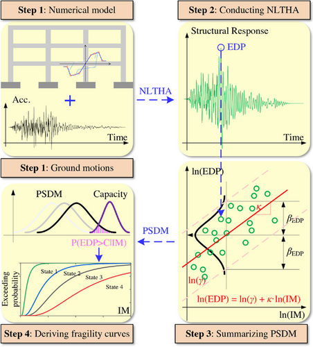
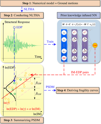
It can be observed that in this procedure, the precision of the derived fragility curves mainly depends on the number of IM-EDP samples. In previous studies, hundreds, even thousands, of deterministic NLTHAs were carried out for this purpose (Cao et al., 2023; de Felice & Giannini, 2010; Rezaei et al., 2023). For step 2, refined finite element models (based on solid or fiber elements) are typically used. Therefore, the computational burden of deriving fragility curves is usually high (Feng et al., 2019). Various prior studies have proposed to use ML as a surrogate to the numerical model to decrease the computational cost, but the number of NLTHA samples (say ) needed for ML training is not much less than that for the conventional approach (Ferrario et al., 2017). Therefore, the proposed PKNN is a viable alternative in step 2 to achieve a meaningful level of computational efficiency.
3.2 Fragility analysis via PKNN
The proposed PKNN can be used for predicting the seismic response of a given structure and significantly accelerate the fragility analysis. As shown in Figure 3 and Figure 2, in the conventional approach, the development of PSDM requires plenty NLTHAs. In our approach, the proposed PKNN can be trained with only a few NLTHAs to generate the IM-EDP pairs. Another major difference between the proposed approach and the other relevant prior work featuring ML-based surrogate models is that, as illustrated in the previous section, the PKNN used here requires far fewer NLTHA samples for training to achieve the same accuracy. A case study is designed and carried out next to comprehensively validate the effectiveness of this proposed approach.
4 CASE STUDY
4.1 Structural modeling
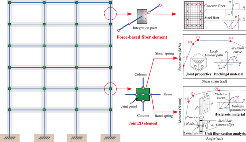
For initially validating the proposed approach, a representative three-span six-story RCF is chosen as the specimen for fragility assessment (Figure 4). The span length of the RCF is 6.3 m. The height for the first story is 4.2 m, and 3.5 m for all other stories. The dimensions of the beam and column cross sections are 350550 mm and 650650 mm, respectively. For the material, type-C30 concrete (14.3 MPa compressive strength) is used. HRB335 steel bars (300 MPa yield strength) and HPB300 bars (270 MPa yield strength) are selected for longitudinal reinforcement and stirrups, respectively. The reinforcement details for beams and columns are given in Figure 4. It should be mentioned that the main purpose of this study is to initially validate the concept of the proposed PKNN-based assessment of a structure. Thus, the simulated RCF here is a commonly used regular frame structure without considering the damage within existing structures (Ning & Xie, 2023; Park et al., 2018). The performance of the proposed approach would be further investigated on more complex scenarios such as an existing RC structure with planar or vertical irregularities in the following studies considering the degradation damages such as corroded reinforcements (Ding et al., 2023; Di Sarno & Pugliese, 2020).

For NLTHA, commonly used fiber element–based modeling approaches are selected and the finite element model is established in well-developed open-source software “OpenSees” (Mazzoni et al., 2006). The model is illustrated in Figure 5. The force-based fiber element with four integration points is adopted for modeling each beam–column component. The constitutive behaviors of unconfined, confined concrete and reinforcing steel are considered in the fiber section (Feng & Ding, 2018). The Joint2D is adopted for modeling beam–column joints. The shear behavior of the joint and the bond-slip behavior of the interface are considered. The strength and stiffness degradation behavior is described by the “Pinching4” model. For the behavior of the bond-slip stress-slip relationship, it is considered in the moment-rotation curve of the corresponding fiber section. More specific details about modeling can be referred to Feng et al. (2018).
For stochastic seismic response prediction and fragility assessment, uncertainties within 13 key structural parameters are considered, and their distribution characteristics are listed in Table 1 in which “Cov.” stands for “Coefficient of Variation.”' These parameters are determined based on previous studies (Ellingwood, 1980; Mirza & MacGregor, 1979a, 1979b; Mirza et al., 1979). Based on this, 320 parameter sets are sampled in order to generate 320 structural models.
| Structural parameter | Distribution | Mean | Cov. |
|---|---|---|---|
| Rebar diameter in columns | Normal | 25 (mm) | .04 |
| Rebar diameter 1 in beams | Normal | 20 (mm) | .04 |
| Rebar diameter 2 in beams | Normal | 18 (mm) | .04 |
| Rebar yielding strength | Log-normal | 378 (MPa) | .074 |
| Rebar elastic modulus | Log-normal | 201000 (MPa) | .033 |
| Rebar hardening ratio | Log-normal | 0.02 (1) | .2 |
| Concrete bulk density | Normal | 26.5 (kN/) | .0698 |
| Core concrete compressive strength | Log-normal | 33.6 (MPa) | .21 |
| Core concrete peak strain | Log-normal | 0.0022 (1) | .17 |
| Core concrete ultimate strain | Log-normal | 0.0113 (1) | .52 |
| Cover concrete compressive strength | Log-normal | 26.1 (MPa) | .14 |
| Cover concrete ultimate strain | Log-normal | 0.004 (1) | .2 |
| Damping ratio | Normal | 0.05 (1) | .1 |
4.2 Ground acceleration selection
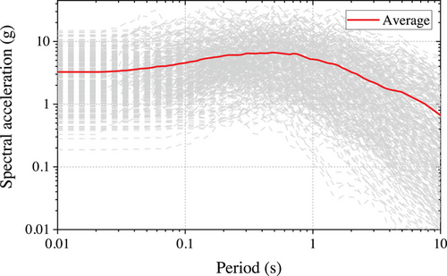
For uncertainties within earthquakes, 160 horizontal ground accelerations containing far-field, near-fault pulse-like ground accelerations recorded at diverse soil conditions are selected from the Pacific Earthquake Engineering Research Center database (Baker et al., 2011). The response spectra are given in Figure 6. After scaling these ground accelerations by factors of 1 and 2, a total of 320 ground acceleration pairs are generated for conducting NLTHA of previously generated 320 structural models.
4.3 Database generation for model training
The NLTHA is carried out by an unconditionally stable explicit solving algorithm “KR-” to alleviate convergence issue (Kolay & Ricles, 2014). Then, the 320 input–output data needed for the fragility analysis and ML model training are extracted from the obtained structural response in NLTHA. The input includes the structural attributes listed in Table 1 and amplitude- and duration-based IM parameters containing PGA, peak ground velocity (PGV), effective design acceleration (EDA), effective peak velocity (EPV), sustained maximum velocity (SMV), velocity spectrum intensity (VSI), characteristic intensity (CI), and Housner intensity (HI). Hence, the input is a 21-dimensional vector. The output of the database is the EDP. For an RCF, EDP is commonly quantified by the MIDR. Meanwhile, based on the theoretical procedure in Figure 5, physical models of the RCFs with 320 structural parameter sets can be established and 320 equations of motion pairing with 320 ground accelerations can be solved via the Newmark algorithm. The similar 320 input–output data can be extracted from the corresponding results and would provide the prior knowledge for the neural network.
4.4 Scenario design for case study
According to the conventional approach given in Figure 2, a baseline PSDM would be derived by pairing the 320 IM-EDP (PGA-MIDR here) pairs via NLTHA for comparison. Then, to illustrate the effectiveness of the proposed approach, only 20% (64) NLTHA generated data are randomly selected for training a PKNN. Then, the trained neural network would be used as a surrogate model for predicting seismic response and facilitating fragility assessment. For ablation tests and comparisons, the conventional neural network–based surrogate model approach is also conducted via the identical training database. In addition to the neural network, the XGboost algorithm is also selected to generate a classic surrogate model to investigate the consequence of algorithm selection, because according to previous studies about predicting seismic response and assessment safety of a structure, the decision tree-based ML algorithm represented by XGBoost mostly outperforms other ML algorithms (Aladsani et al., 2022; Mangalathu et al., 2020; Mangalathu & Jeon, 2019). As for deep learning algorithms, they were proven to be not more adept on tabular data than decision tree–based models. Mostly the gradient-boosted tree ensembles still outperform deep learning models on supervised learning tasks on tabular data (Borisov et al., 2022; Shwartz-Ziv & Armon, 2022). The data size treated in this case is small, which is also not suitable for a deep learning model. Thus, the deep learning algorithms are not adopted in the case study.
The scenarios for the entire case study are summarized in Table 2 where “PK” stands for prior knowledge. It should be noticed that S1 is the baseline for comparison and S4 represents that the neural network is only trained via stage 1 of Algorithm 1 without any NLTHA data in order to illustrate the pure effect of a physical model. For all ML models trained in this study, their hyperparameters would be optimized via mature Bayesian optimization algorithms. For specific processes, one can be referred to Akiba et al. (2019).
| Scenario | Nonlinear time history analysis (NLTHA) data | Prior knowledge (PK) | Machine learning (ML) model |
|---|---|---|---|
| S1 | 100% (320) | N/A | |
| S2 | 20% (64) | Neural network | |
| S3 | 20% (64) | Xgboost | |
| S4 | 0% (0) | Neural network | |
| S5 | 20% (64) | Neural network |
5 RESULTS AND DISCUSSION
5.1 Seismic response prediction of a structure
The accuracy of the predicted response within each scenario is discussed first. The comparison between actual and predicted seismic MIDR of the RCF is displayed in Figure 7. In Figure 7a,bd, the points circled out represent the training set for the model. The accuracy index commonly used is also given in Figure 7 where R represents the coefficient of determination and MSE is defined as before.

According to the distribution of the scatter of points, it can be seen that among the four models, the PKNN model used in S5 exhibits the best regression performance, which can also be proved by the accuracy indexes. The improvement over the other model is evident while the least improvement ratio on R and MSE reaches 13.94%, and 22.38%, respectively. Though the neural network trained in S2 has a high accuracy on the training data, the overall prediction accuracy is poor, which implies the model has been overfitted. A similar overfitting phenomenon can also be seen in S3, though the value of the accuracy indexes in S3 is close to the index performance in S5, which mainly owing to its good prediction when MIDR 0.25. However, the prediction of the XGBoost model in S3 seems to be restrained under a certain value, and for MIDR larger than.05 its prediction error is extremely high. This is mainly caused by the nature of the XGBoost algorithm, as a tree-based ML model that inherently cannot make predictions outside the valuing range of the training database, and most of the MIDR in the training data is less than. 25 (Arik & Pfister, 2021). Thus, when the training data are not adequate, a conventional ML-based surrogate model may not work as usual no matter which algorithm is used. As for S4, the whole prediction resulting from the physical model is poor and entirely underestimates the MIDR. Based on these results, it can be proved that on one hand the good performance of PKNN is not simply contributed by the small training database from NLTHA or the data from the physical model, and on the other hand, the effectiveness of the proposed two-stage training strategy of PKNN on response prediction is validated.
Although the performance of PKNN on seismic response prediction exceeds all other models, its absolute accuracy is not ideally high. Its performance on the downstream task such as fragility assessment is still unknown. Then, the performance of applying the PKNN in fragility assessment is further discussed.
5.2 Fragility assessment
Based on four generated response prediction models in the last section, the PGA-MIDR (IM-EDP) pair data for fragility assessment can be generated. The generated PGA-MIDR data and corresponding PSDMs are illustrated in Figure 8 where “LR” stands for “linear regression.” Similarly, in Figure 8, the data points circled in black represent the training data for S2, S3, and S5. One interesting thing that needs to be pointed out is that the ln(PGA) value of all training data is larger than −3, which means the extrapolating capacity of the trained surrogate models would be examined when the prediction falls in the range ln(PGA) −3.
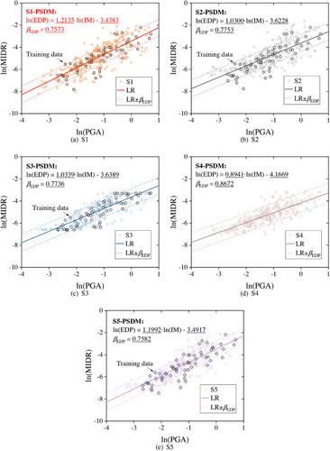
According to the distributions of the scatter points shown in Figure 8, it can be seen that the data generated in S2 differs a lot from that in S1 when ln(PGA) is less than −3. A similar scene can also be found in S3 and moreover, the predicted MIDRs are almost constant as ln(PGA) −3. As found in the last section, this phenomenon is also the result of poor extrapolation capacity of the trained surrogate model in S2 and S3. Thus, when the training data are not adequate, conventional ML-based surrogate models still cannot work in fragility assessment. As for S4, according to the slope of the regressed linear model, the data generated in S4 has a global bias, which mainly comes from the theoretical simplifications of the physical model. As for S5, it can be seen that the distribution of data highly resembles the data in S1. Though the PKNN in S5 is trained on the same database used in S2 and S3, the poor extrapolation issue does not appear when ln(PGA) −3. This mainly owes to the prior knowledge from the theoretical model. Despite the physical model not being accurate, as displayed in S4, it can provide good prior knowledge on the entire prediction space to the ML model.
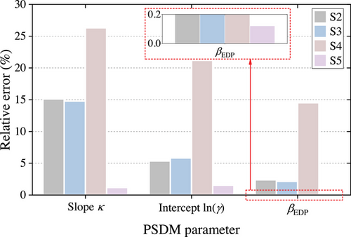
For further quantifying the performance of each approach, the relative difference between the baseline PSDM's parameters in S1 and others is summarized in Figure 9. It can be seen that the PSDM in S5 is the closest one to the baseline with merely 1.18%, 1.55%, and 0.12% relative error on slope, intercept, and , respectively. For comparison, it can be seen that S4 is the worst, which also implies that the original physical model cannot accurately describe the seismic behavior of the structure. In the meantime, the PSDMs in S2 and S3 also severely deviate from the baseline PSDM. However, based on the identical database, a quite accurate PSDM could be obtained via the proposed PKNN-based approach. This strongly validates its effectiveness.
Furthermore, the fragility curves derived from five PSDMs are given in Figure 10. For fragility assessment, four widely adopted performance levels provided by federal emergency management agency are used, where 0.2%, 1%, 2%, and 4% MIDR are used to describe slight, moderate, extensive, and complete damage states, respectively (Feng, Sun, et al., 2023; Prestandard, 2000). It can be seen that in four performance levels, the fragility curves derived in S2, S3, and S4 have a large deviation. In contrast, the fragility curves in S5 almost coincide with those baseline curves in S1.

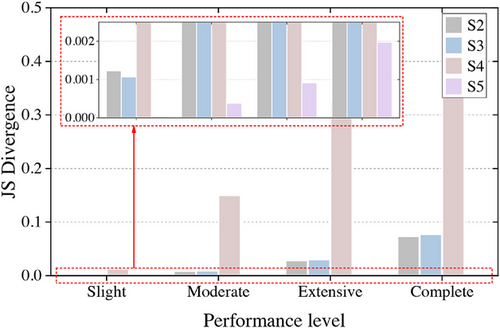
The JS divergence results between baseline fragility curves and others are given in Figure 11. It can be seen that for all scenarios, the difference between baseline fragility results and others would rise under a more severe performance level. Meanwhile, the fragility results in S5 are the closest to the baseline no matter which performance level is considered. With the help of JS divergence as the index, it is proved that the precision of the proposed approach in S5 is significantly better than the others.
All in all, these results strongly demonstrated the effectiveness of the proposed PKNN-based fragility assessment approach. Although the PKNN's accuracy on the seismic response prediction is not perfect, it can still be applied in fragility assessment with rather good performance. It was proved that comparable assessment results could be obtained based on only 20% computational cost.
5.3 Influence of NLTHA data amount used in PKNN
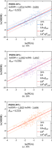
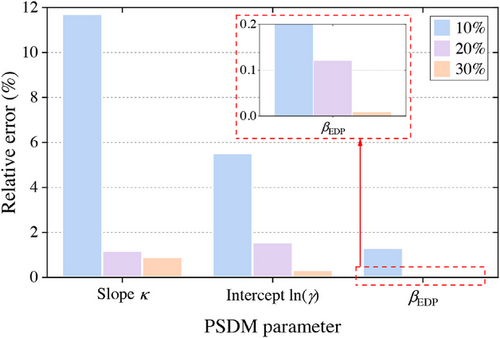
To further investigate the influence of the NLTHA data number on the proposed PKNN-based method, the assessment based on the proposed approach with 10% (32) and 30% (96) NLTHA data is carried out. First, the generated PGA-MIDR data and derived PSDMs from various NLTHA data are present in Figure 12 where superscript “B” represents the baseline model from the previous S1. It can be seen that the difference between the derived PSDM and the baseline would evidently decrease as the amount of NLTHA data for model training increases. Moreover, the degree of improvement would seemingly become saturated, because the gap between cases with 10% and 20% NLTHA data is more dramatic than that between cases with 20% and 30% data. Similarly, the relative error of these three PSDMs in comparison with the baseline is given in Figure 13. It can be seen that the model generated from 30% NLTHA data attains the best relative error performance with only 0.91%, 0.33%, and 0.01% on three PSDM parameters. It is also demonstrated that the improvement caused by introducing more NLTHA data would gradually decrease.
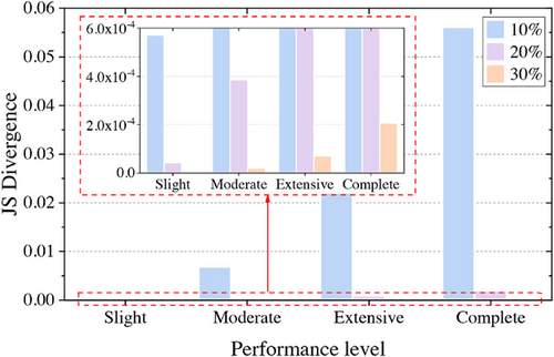
The fragility results are also derived from these PSDMs as given in Figure 14. A similar trend can be observed that with more NLTHA data, the derived fragility curves would be closer to the baseline. To better quantify this trend, JS divergence between them is displayed in Figure 15. It is illustrated more clearly that more NLTHA data could effectively promote the precision of the fragility results but the gain from the increased data would lessen. Therefore, when applying the proposed approach, an optimal balance between the demanded accuracy and the acceptable computational cost should be carefully considered.

6 CONCLUSION
- (1) The proposed PKNN has been initially proven to be able to accurately capture the mapping relationship between structural, and seismic attributes and the corresponding structural response such as MIDR via a rather small number of numerical simulations. Consequently, it can be used to enhance the overall efficiency of the structural fragility analyses.
- (2) In the case study, compared with the conventional ML-based surrogate model, the PKNN would provide much more accurate MIDR prediction of an RC frame structure (relative error less than 1%) and reliable fragility curves when only 20% numerical simulated MIDR data needed for the conventional approach are used for training.
- (3) By introducing more numerical simulation data in training the PKNN, the relative error between corresponding fragility assessment results and the accurate results would gradually decline, while the gain from increasing simulation data would also decline. Thus, in practice for achieving a relatively precise result with high efficiency, the simulation data amount for training the proposed PKNN should be carefully selected.
In this study, the proposed approach was only validated on a regular RC frame structure via fiber element–based numerical models. In order to investigate its generalizability and scalability, further research will focus on the application of the PKNN on response prediction and fragility assessment of more complex existing structures with planar or vertical irregularities such as shear wall structures and bridges. More refined numerical models like shell and solid element-based models would also be utilized for investigation.
ACKNOWLEDGMENTS
The corresponding author acknowledges financial support from the National Key Research and Development Program of China (Grant Numbers 2021YFB1600300, 2022YFC3803004), National Natural Science Foundation of China (Grant Number 52078119), Natural Science Foundation of Jiangsu Province (Grant Number BK20211564), and Fundamental Research Funds for the Central Universities, CHD (300102213209).


