Various earthquake early warning (EEW) methodologies have been proposed globally for speedily estimating information (i.e., location, magnitude, ground-shaking intensities, and/or potential consequences) about ongoing seismic events for real-time/near real-time earthquake risk management. Conventional EEW algorithms have often been based on the inferred physics of a fault rupture combined with simplified empirical models to estimate the source parameters and intensity measures of interest. Given the recent boost in computational resources, data-driven methods/models are now widely accepted as effective alternatives for EEW. This study introduces a highly accurate deep-learning-based computational framework named ROSERS (i.e., Real-time On-Site Estimation of Response Spectra) to estimate the acceleration response spectrum (S_a(T)) of the expected on-site ground-motion waveforms using early non-damage-causing early p-waves and site characteristics. The framework is trained using a carefully selected extensive database of recorded ground motions. Due to the well-known correlation of S_a(T) with structures’ seismic response and resulting damage/losses, rapid and accurate knowledge of expected on-site S_a(T) values is highly beneficial to various end-users to make well-informed real-time and near-real-time decisions. The framework is thoroughly assessed and investigated through multiple statistical tests under three historical earthquake events. These analyses demonstrate that the overall framework leads to excellent prediction power and, on average, has an accuracy above 85% for hazard-consistent early-warning trigger classification.

1 INTRODUCTION

Earthquake early warning (EEW) computational frameworks are generally developed to define different alert levels for life and asset protection from earthquake-induced ground shaking before reaching a given target site. Research on EEW is mainly oriented to efficiently provide timely and accurate warnings and support risk-management decision-making during an earthquake event, that is, from the time of fault rupture to when the ground shaking ends at the target site. In a real-time setting, EEW utilizes information from the fast-traveling longitudinal p-waves (characterized by low-amplitude and generally non-damaging) of the arriving earthquake waveform to trigger alerts for preparing against the high-amplitude (destructive) transverse s-waves. Typically, p-waves are 1.7 times faster than s-waves in any given material (Kramer, 1995). EEW systems exploit this time lag between the arrival of the p-waves and s-waves to predict various parameters of interest for real-time decision-making purposes.

EEW systems mainly consist of two general sub-classes: (1) regional and (2) on-site. A regional EEW system is a network-based system consisting of seismic sensors installed near a seismic source zone. When an earthquake is detected, a regional EEW system uses the information from the initial seconds of the ground motions (mainly p-waves) recorded at several stations close to the source to alert target sites farther from the source. The alert is generally based upon the rapid estimation of the earthquake location and magnitude, which are then used as inputs to pre-calibrated ground-motion models (GMMs). These GMMs estimate the distribution of intensity measures (IMs) of the expected ground-motion at a given site (Bhardwaj et al., 2016; Cremen & Galasso, 2020; Li et al., 2013; Mu & Yuen, 2016). This type of approach leads to large variabilities in the IM estimates due to the propagation of uncertainty for estimating source parameters (location and magnitude) and the uncertainties, both epistemic and aleatory, in GMMs (Iervolino et al., 2009). Various regionals EEW methodologies attempt to directly predict ground-motion IMs at target sites bypassing the source parameter estimation (Hoshiba & Aoki, 2015; Münchmeyer et al., 2020). However, these approaches are not ideal for regions in the vicinity of a seismic source (generally known as blind zones) due to multiple reasons such as longer computation times and the requirement of a dense array of sensors, limiting the handing of maximal information in a real-time setting. Some studies, such as Panakkat and Adeli (2009) and Rafiei and Adeli (2017), have also proposed detailed methodologies to forecast an earthquake event parameter (such as location), weeks to days before its occurrence (such methods fall under a separate class of short-term earthquake forecasting frameworks, known as operational earthquake forecasting [OEF]). Panakkat and Adeli (2008) presented several advances made in OEF methods.

On the other hand, an on-site EEW system is a standalone system based on a single sensor (or a small array of sensors) located in the proximity of the target sites. Within this setting, the characteristics of early p-waves observed on-site are used to estimate the earthquake source parameters or the IMs of the expected ground motion that mainly comprise the late s-waves and surface waves at the same site. This approach is specifically beneficial for sites located within blind zones as the expected shaking levels are estimated for the same site observing the ground-motion, thereby requiring minimum time. Most of the on-site EEW approaches utilize pre-trained parametric or non-parametric models to estimate amplitude-based, energy-based, frequency-based, and duration-based IMs using the initial seconds of the ground-motion waveforms in real-time (e.g., Brondi et al., 2015; Caruso et al., 2017; Colombelli & Zollo, 2015; Hsu et al., 2013; Münchmeyer et al., 2020; Wu & Kanamori, 2008). However, the development of such methods requires careful attention in terms of using IMs that provide (statistically) sufficient and efficient information for real-time decision-making. For instance, most of the existing on-site EEW algorithms (such as Caruso et al., 2017; Colombelli & Zollo, 2015; Hsu et al., 2013; Münchmeyer et al., 2020) are trained to estimate scalar quantities such as peak ground acceleration (PGA) or peak ground velocity (PGV). These only provide information about the shaking of the ground and not their potential consequences on the structures/infrastructure in the area. The use of poorly informative IMs can, in turn, lead to sub-optimal EEW decision-making (i.e., increased occurrences of false and missed EEW alarms) with the current approaches. Such insufficient EEW frameworks can have a detrimental impact on the socio-economic conditions of the affected region. False positives (cases in which a wrong prediction of high shaking is made, i.e., false alarms) can result in long downtimes and panic. On the other hand, false negatives (cases in which a wrong prediction of low shaking is made, i.e., missed alarm) have self-evident consequences in terms of economic losses and even casualties. Furthermore, false negatives severely increase a community's vulnerability since a population convinced that it is likely to be warned before high levels of shaking are likely to be less prepared. Such cases are already noticed in research studies (Meier, 2017; Minson et al., 2019; Wald, 2020), which have criticized the uses of EEW systems and demonstrated mistrust in EEW. Studies such as those by Wu et al. (2013) and Hsu et al. (2016) proposed relevant approaches that can assist EEW in reducing false alarms. In particular, Wu et al. (2013) proposed an earthquake probability-based automated decision-making framework. The framework uses basic decision theory and existing cost–benefit analysis procedure (i.e., based on conventional GMMs) to suggest a general decision criterion in EEW. Coupling such decision-making methods with an accurate IM prediction method (as proposed in this study) can lead to more robust EEW systems.

In the field of performance-based earthquake engineering, the acceleration response spectrum, S_a(T), is a widely used IM that can effectively integrate the characteristics of the ground-motion waveform (such as amplitude, frequency content, etc.) with the dynamic behavior of a structural system idealized as a single-degree-of-freedom system (SDoF; Bazzurro et al., 1998; Vamvatsikos & Allin Cornell, 2002). An accurate estimation of the ground-motion S_a(T) values in real time can help stakeholders better design engineering applications of EEW, including those relying on risk-informed decision support systems (Cremen & Galasso, 2021). Recently, Iaccarino et al. (2020) and Jozinović et al. (2020) proposed data-driven methods (such as mixed-effect model and convolutional neural networks, respectively) to obtain S_a(T) values for few periods using initial seconds of the arriving ground motions; however, based on the results presented in their work, the frameworks’ accuracy and robustness to work efficiently in real time could be further improved.

This paper contributes to extending the objectives of current EEW frameworks to be accurate, timely, and both structurally- and ground-motion- informed. In particular, this study proposes a highly precise and novel on-site EEW framework named real-time on-site estimation of response spectra (ROSERS) developed using a deep neural network (DNN) and a variational autoencoder (VAE). The framework uses site characteristics (SC) of the recording station(s) and an IM vector (representing amplitude, energy, duration, and frequency content) of the initial 3 s of the arriving ground-motion (after detection of p-waves) to estimate a vector of PGA (PGA is also referred to S_a(T = 0)) and spectral ordinates (i.e., the S_a(T) spectrum for 95 SDoF periods (T)) for the expected on-site complete ground-motion waveform. The framework utilizes a trained feed-forward DNN to concurrently estimate a set of two mathematical-representative latent variables using the SC and the considered IM vector as inputs. The obtained latent variables are then inputted to a trained VAE decoder to develop the 96-period S_a(T) spectrum (including PGA) of the expected on-site ground-motion. The framework is evaluated through rigorous statistical tests and testbed studies for three historic earthquakes events. Hence, apart from utilizing a more structurally informed IM as a target decision variable for EEW, this study utilizes an advanced neural-network approach to optimally conduct dimensionality reduction of the S_a(T) spectrum into surrogate latent variables that can be practically used in real time. Furthermore, using data-driven and deep-learning-based methods minimizes the assumptions involved in the model development and makes the framework flexible and easily re-trainable. In addition, the high dimensional interpolative and extrapolative nature of DNNs makes this study more robust than non-deep learning-based and traditional methods (Gustafson et al., 1990; Xu et al., 2021). The proposed framework is observed to perform well on the used dataset, and based on the findings of this paper, it can be highly beneficial to advance EEW research and support various end-users.

The paper starts by introducing the proposed framework and its key implementation steps. Then, the considered ground-motion database, algorithms, and models used to develop the framework are explained, and the results of various statistical tests are presented. Finally, the proposed framework is illustrated by applying it to three historical earthquake events recorded in California, used as testbeds. The illustration is conducted to test the performance of the proposed framework in hazard-consistent alarm triggering.

2 PROPOSED FRAMEWORK

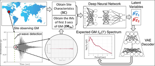
The proposed ROSERS framework is illustrated in Figure 1. A digital recording station continuously monitors ground shaking at a given location. As the seismic sensor detects the initial p-waves of the arriving ground-motion (e.g., Akazawa, 2004; Kalkan, 2016; Sleeman & van Eck, 1999), the ROSERS framework stands by to receive 3 s of the incoming ground-motion. While any picker algorithm can be used to detect p-waves arrival, this study uses the P_PHASEP_ICKER algorithm by Kalkan (2016). ROSERS utilizes the first 3 s of the observed ground-motion in real time to compute a vector of seven intensity measures denoted as IM_3s. The vector IM_3s correspond to the amplitude, energy, frequency, and significant duration of the initial 3 s of the ground-motion waveform after detection of p-waves. The computed IM_3s is combined with the vector of site characteristics (denoted as SC) of the recording station, known a-priori. The obtained IM_3s and SC are then used as inputs to a pre-trained feed-forward DNN estimating two mean latent variables $(\widehat {{\mu _{{z_1}}}}$ and $\widehat {{\mu _{{z_2}}}})$ , which are then cascaded to a pre-trained VAE decoder. It should be noted here that the two latent variables are not physically derived but represent a two-dimensional statistical surrogacy of the complete ${S_a}( T )$ spectrum, which is obtained by training a VAE. The VAE decoder transforms the estimated mean latent variables ( $\widehat {{\mu _{{z_1}}}}$ and $\widehat {{\mu _{{z_2}}}}$ ) into the vector of PGA and 95-period S_a(T) spectrum (denoted as S_a). The obtained S_a vector can be utilized by various end-users/stakeholders to informatively alert a community through risk-informed EEW decision support systems, develop shakemaps, perform structural control, and other similar applications in real-time (Cremen & Galasso, 2021). The estimation of the S_a vector through ROSERS takes less than 1 s on average, thereby providing end-users with an ample amount of time for decision-making.

Details are in the caption following the image — **FIGURE 1**
Open in figure viewer PowerPoint

Illustration of the real-time on-site estimation of response spectra (ROSERS) framework. The illustration flows from left to right. The implementation of this ROSERS framework, on average, takes ∼0.75 s on a modern personal computing machine

3 GROUND-MOTION DATABASE

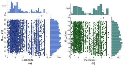
The framework is developed and trained using the recorded ground motions available in the comprehensive database of the Next-Generation Attenuation West version 2 (NGA-West2) project (Ancheta et al., 2014). The database utilized in this study consists of 13,916 ground-motion components from 277 seismic events recorded worldwide and are processed based on the recommendations of (Boore & Bommer, 2005). It is worth noting that ground motions in real time are generally not processed in the same manner, and the processing usually involves the use of simplistic techniques such as trend removals and low-pass and high-pass filtering (Caruso et al., 2017; Hsu et al., 2013). However, this assumption is not expected to significantly change the proposed framework's predictive performance: The data-driven nature of the artificial neural networks, with sufficient training, can quickly make the framework adapt to any minor deviances and noise (Borodinov et al., 2019; Jumper et al., 2021). The moment magnitude (M) and closest rupture distance (R_rup) metadata of the considered database is provided in Figure 2a. Other details of the metadata can be obtained from (Fayaz et al., 2021). As can be observed from Figure 2a, the database is skewed toward events with $M \le$ 5.5. Hence, in this study, the ground motions with $M \le$ 5.5 (majority class) are undersampled (Lemaitre et al., 2017) such that the number of ground motions with $M \le$ 5.5 and $M >$ 5.5 is equivalent while maintaining the distributions of ${R_{rup}}$ and site's average shear-wave velocity of the soil up to 30 m ( ${V_{s30}}$ ). This results in 6,392 ground-motion components whose event data is presented in Figure 2b. The distributions for ground motions with $M \le$ 5.5 and $M >$ 5.5 are observed to be similar. The bimodal shape of the M histograms is inherited in the data as not enough seismic recordings are available for 5 $\le M \le$ 6. For the obtained ground motions, their acceleration response spectra at 96 periods (S_a(T) for periods from 0 to 5 s) is computed.

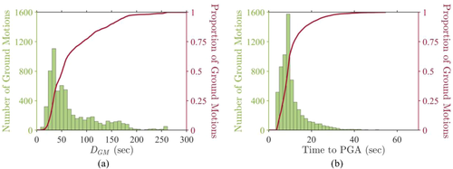
To assess the ground-motion time used by the proposed framework (i.e., initial 3 s after the detection of p-waves) with respect to the ground-motion duration for the undersampled dataset, the overall duration ( ${D_{GM}}$ ) and time to PGA after detection of p-waves is computed. To avoid the inclusion of zeros and very small acceleration values (< 10^–5 g) in the computation of ${D_{GM}}$ (which are padded while processing of ground motions in NGA-West2), ${D_{GM}}$ is computed by obtaining the time difference between attainment of 99.9% and 0.1% of ${I_a}$ (similar to the computation of significant duration ${D_{5 - 95}}$ ; Kramer, 1995). Figure 3a,b shows the ${D_{GM}}$ and time to PGA of the undersampled ground-motion dataset, respectively. It is observed that ${D_{GM}}$ has a mode of about 40 s, and the time to PGA has a mode of about 30 s. This means that the predictions made within the initial 3 s of the on-site ground motions (after detection of p-waves) can still allow an ample amount of warning time for decision-making. Thus, the proposed framework can assist in taking real-time risk mitigation actions such as the start of evacuation procedures/move to safer locations within a structure, automatic emergency responses, road closures, and so forth, before the arrival of the peak acceleration and before shaking ends. This further indicates the framework's usefulness to perform well in a real-time setting.

3.1 p-phase arrival-time picker

Though the ground motions in the NGA-West2 database are already processed, the ground-motion records do not necessarily start with p-waves and may contain additional zeros and early station noise in the recordings. Hence it is crucial to detect the p-waves in the ground motions to develop the proposed EEW framework. This study obtains the p-waves arrival time in the ground-motion time histories using an automated p-phase picker approach developed by Kalkan (2016). Unlike other approaches (Akazawa, 2004; Sleeman & van Eck, 1999), the proposed method for picking p-phase arrival times in single-component acceleration or broadband velocity records does not require any detection interval or threshold setting. The algorithm P_PHASEP_ICKER obtains the response of an SDoF oscillator with viscous damping subjected to the input ground-motion and then measures the dissipated damping energy. The rate of change (power) of the measured damping energy is then used to pick p-wave phases (Kalkan, 2016). The SDoF oscillator is developed to possess a short natural period and consequently a high resonant frequency. This is done to ensure that the natural frequency of the SDoF is higher than the frequencies mostly observed in seismic waves, which prevents the effects of resonance. Phases angles are maintained as the SDoF is provided with a high damping ratio (60% of critical) at which the frequency response reaches the Butterworth maximally flat magnitude filter. The relative input energy imparted to the oscillator by the input ground-motion is converted to elastic strain energy and then dispelled by the damping element as damping energy. The computed damping energy generates a smooth envelope over the duration of the seismic ground-motion. The envelope is close to zero at the beginning of the signal before the arrival of p-phase and builds up swiftly with the arrival of the p-wave. The considerable change in the damping energy function at the onset of the p-wave is used to track and pick the arrival of p-phase. The P_PHASEP_ICKER particularly detects the onset of p-phase using the histogram method (Anon, 2011; Solomon et al., 2001). The histogram method is used as the picking algorithm, as it does not require any detection interval or threshold settings. The 6,392 ground-motion components are analyzed using the P_PHASEP_ICKER algorithm to obtain their corresponding p-wave arrival time, and only the ground-motion time histories after p-wave arrival are considered for the computation of IM_3s and further analysis in this study.

4 COMPONENTS OF THE ROSERS FRAMEWORK

This section presents the details of the models used in the proposed framework and the statistical analysis results conducted to test their prediction power. The section first explains the details of the VAE model that is used to project the ${{\bm{S}}_{\rm{a}}}$ vector into the two latent-variable space. Then the DNN model used to estimate the mean of the two latent variables is discussed; finally, the hierarchical mixed-effects regression of the residual is described. For each sub-section, the model is explained first, and then its prediction power is described.

4.1 Variational autoencoder

The ${{\bm{S}}_a}$ vector computed for the 6,392 ground-motion components for the 96 periods is used as input to be reconstructed in the VAE (Kingma & Welling, 2019). The VAE is bottlenecked to have two independent normally distributed latent variables (denoted as ${z_1}$ and ${z_2}$ with means ${\mu _{{z_1}}}$ and ${\mu _{{z_2}}}\$ and variances $\sigma _{{z_1}}^2$ and $\sigma _{{z_2}}^2$ , respectively) in the sampling layer. A two-dimensional latent variable space is used as it results in a good trade-off between higher reconstruction power and a lower number of latent dimensions. The neural network-based VAE is trained through cross-validation using a randomly split 80% of the dataset while the remaining 20% is used as the final test set. The training and testing of the VAE are performed using a log transformation of ${S_a}( T )$ as the ground-motion IMs are generally observed to be lognormally distributed (Zarrin et al., 2020). VAE provides a probabilistic approach to describe a vectorial observation in their latent variable space. This is done using a neural network-based encoder (recognition model) trained in conjunction with a neural network-based decoder (generative model) that can use the latent variable space to reconstruct the observations. This means that the encoder describes a probability distribution for each latent attribute from which values are randomly sampled to be fed into the decoder that is expected to accurately reconstruct the input. Hence, the latent space is essentially compelled to possess continuous and smooth representations. Consequently, nearby values in the latent space correspond to similar reconstructions using the decoder. It is worth mentioning that while there are other approaches to this aim, such as principal component analysis, singular value decomposition, regular autoencoders, and so forth, such methods do not necessarily provide a continuous probabilistic space of reduced dimensions (i.e., latent variables) along with such high accuracy and reconstruction power.

The underlying idea of training the VAE relies on the basic Bayes’ rule given in Equation (1), where

{\bm{x}}

represents the true vector of input variables and

{\bm{z}}

represents the latent variable space. Due to its intractability,

p( {\bm{x}} )

can be estimated using variational inference (Blei et al., 2017). This relies on estimating

p( {{\bm{z}}|{\bm{x}}} )

by another distribution

q( {{\bm{z}}|{\bm{x}}} )

, which is defined such that it has a tractable distribution. By defining

q( {{\bm{z}}|{\bm{x}}} )\

such that it is very similar to

p( {{\bm{z}}|{\bm{x}}} )

, it can be used to perform approximate inference of the intractable distribution. This is done by minimizing the Kullback and Leibler (KL) divergence (Kullback & Leibler, 1951) between

q( {{\bm{z}}|{\bm{x}}} )

and

p( {{\bm{z}}|{\bm{x}}} )

shown in Equation (3), where the KL divergence between any two distributions

p

and

q

can be computed using Equation (2). The minimization process of Equation (3) can be conducted by maximizing the expression given in Equation (4) where

{E_{q( {{\bm{z}}|{\bm{x}}} )}}\log p( {{\bm{x}}|{\bm{z}}} )

represents the reconstruction likelihood, and

{\rm{KL}}[q( {{\bm{z}}|{\bm{x}}} )||p( {\bm{z}} )]

ensures that the learned posterior distribution

q( {{\bm{z}}|{\bm{x}}} )

is similar to the prior distribution

p( {\bm{z}} )

, which is assumed to be a standard Gaussian distribution

( {\sim N( {0,1} )} )

for each latent variable.

{E_{q( {{\bm{z}}|{\bm{x}}} )}}\log p( {{\bm{x}}|{\bm{z}}} )

is the mean-squared error (L2 loss) between

{\bm{x}}

and

{\bm{\hat{x}}}

(Kingma & Welling, 2019).

\begin{equation}p\ \left( {{\bm z}{\rm{|}}{\bm x}} \right) = \frac{{p\left( {{\bm x}{\rm{|}}{\bm z}} \right)p\left( {\bm z} \right)}}{{p\left( {\bm x} \right)}}\end{equation}

(1)

\begin{equation}{\rm{KL}}[q{\rm{|}}p{\rm{]}} = \mathop \sum \limits_{i = 1}^N q\left( {{y_i}} \right){\rm{log}}\frac{{q\left( {{y_i}} \right)}}{{p\left( {{y_i}} \right)}}\end{equation}

(2)

\begin{equation}{\rm{min}}|{\rm{KL}}[q\left( {{\bm{z}}|{\bm{x}}} \right)\left| {|p\left( {{\bm{z}}|{\bm{x}}} \right)]} \right|\end{equation}

(3)

\begin{equation}{\rm{max}}|{E_{q\left( {{\bm{z}}|{\bm{x}}} \right)}}\log p\left( {{\bm{x}}|{\bm{z}}} \right) - {\rm{KL}}[q\left( {{\bm{z}}|{\bm{x}}} \right)\left| {|p\left( {\bm{z}} \right)]} \right|\end{equation}

(4)

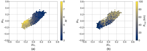
The proposed VAE consists of eight layers in the encoder and decoder (including the input and output layers) with a total of 850 neurons and two-dimensional latent variable space. The VAE is trained with the train set in epochs using the Adaptive Moment Estimation (Adam) (Kingma & Ba, 2014) optimizer and early stopping (Chollet, 2018) regularization. The means of the two latent variable distributions are presented in Figure 4, where the colors of the markers represent the magnitude (M) of the seismic event (Figure 4a) and rupture distance ( ${R_{rup}}$ ) of the station site (Figure 4b). It can be observed from Figure 4a that smaller magnitudes (M < 5.5) tend to have ${\mu _{{z_1}}}$ > 0 and ${\mu _{{z_2}}}$ > 0, and larger magnitudes ( $M$ > 5.5) tend to have ${\mu _{{z_1}}}$ < 0 and ${\mu _{{z_2}}}$ < 0. In general, ${\mu _{{z_1}}}$ and ${\mu _{{z_2}}}\$ tend to decrease with an increase in magnitudes. Similarly, from Figure 4b, it can be observed that smaller rupture distances ( ${R_{rup}}$ < 45 km) tend to have ${\mu _{{z_1}}}$ < 0 and ${\mu _{{z_2}}}$ < 0, and larger rupture distances ( ${R_{rup}}\$ > 45 km) tend to have ${\mu _{{z_1}}}$ > 0 and ${\mu _{{z_2}}}$ > 0. In general, ${\mu _{{z_1}}}$ and ${\mu _{{z_2}}}$ tend to increase with an increase in rupture distances. This shows that the latent variables have an inverse attenuation relation with the $M$ and ${R_{rup}}$ , as they decrease with an increase in $M$ and decrease in ${R_{rup}}$ .

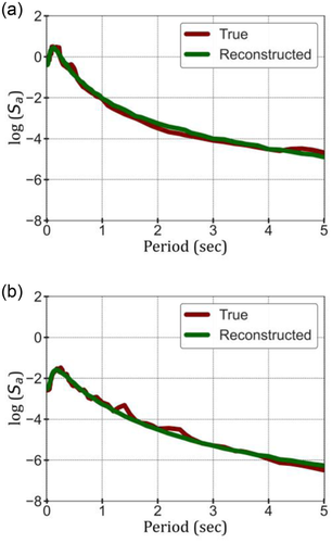
Furthermore, Figure 5a,b shows two examples of the true ${{\bm{S}}_{\rm{a}}}$ spectrum and reconstructed $\widehat {{{\bm{S}}_{{\bf a}}}}$ spectrum for different levels of shaking intensities. It can be observed from the figures that the trained VAE performs well in reconstruing the spectrum using the mean latent variables without any clear bias toward any level of shaking.

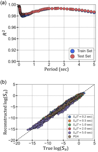
The overall results of the developed VAE are presented in Figure 6a,b. The coefficient of determination R² between the true ${{\bm{S}}_{\rm{a}}}$ and reconstructed $\widehat {{{\bm{S}}_{\rm{a}}}}$ for the 96 periods for both train and test sets are presented in Figure 6a. R² for all periods is observed to be above 0.98, demonstrating excellent reconstruction power of the developed VAE with minimal bias and variance. This can be further observed from Figure 6b, where the true versus reconstructed ${S_a}( T )$ are presented for periods 0.2, 0.5, 1, 2, 5, and 0 s (PGA). For all the cases, it is observed that the true vs. reconstructed ${S_a}( T )$ follow the identity line (1:1) very closely for all ranges of values, demonstrating no bias and high reconstruction power of the VAE. Even with just a visual comparison (since a comparable goodness-of-fit measure is not reported in the reference studies) of Figure 6b with other state-of-practice EEW frameworks (Münchmeyer et al., 2020; Caruso et al., 2017; Colombelli & Zollo, 2015; Hsu et al., 2013), the superiority of the proposed framework can be observed. Based on Figure 6a,b, it is clear that the mean latent variables ${z_1}$ and ${z_2}$ can adequately reconstruct the $\ {{\bm{S}}_{\rm{a}}}$ using the VAE decoder. Hence, if one can estimate the mean latent variables ${\mu _{{z_1}}}$ and ${\mu _{{z_2}}}$ of the ground motions accurately, the trained VAE decoder can be used to transform the estimated latent variables into the ${{\bm{S}}_{\rm{a}}}$ . It is worth mentioning that, although a VAE is primarily used as a generative model (Gorijala & Dukkipati, 2017), the idea of dimensionality reduction coupled with a VAE's requirement to possess continuous and smooth representations of latent variables makes it a perfect candidate for the real-time estimation of the ${{\bm{S}}_{\rm{a}}}$ of the incoming ground motions. The latent variables for new observations can be easily interpolated and extrapolated, leading to good construction of the corresponding spectrum. Also, the utilization of the surrogacy and dimensionality reduction leads to the estimated ${{\bm{S}}_{\rm{a}}}$ that is inherently cross-correlated as the prediction is made jointly for the complete ${{{S}}_{{a}}}( T )$ spectrum at 96 periods.

4.2 Estimation of latent variables

In a real-time setting, to construct the ${{\bm{S}}_{\rm{a}}}$ of the expected ground-motion, it is essential to accurately estimate the mean latent variables ${\mu _{{z_1}}}$ and ${\mu _{{z_2}}}$ , which can then be used in the VAE decoder. To allow ample on-site warning time during the occurring ground-motion, which can last up to 1 to 2 min in some conditions (Figure 3a; Fayaz, et al., 2020), only a few early seconds of the arriving waveform can be practically used for any predictions and early warning. Various initial time windows (ranging from 1 to 10 s) after detection of p-wave arrival were considered for computing the considered ground-motion IMs. For each time window, the mean latent variables were used as the target variables for linear regression, and the computed seven IMs and two site characteristics were used as the predictors. During this exercise, the time window of 3 s was observed to be a good trade-off between the prediction power to estimate ${\mu _{{z_1}}}$ and ${\mu _{{z_2}}}$ and the requirement of a short time window. Prediction power was decided in terms of the average R² ( $R_{Avg}^2$ ) obtained for estimating ${\mu _{{z_1}}}$ and ${\mu _{{z_2}}}$ ; it was observed that IMs obtained from time windows longer than 3 s did not lead to a significant increase in the average R². Figure 7 presents the observed $R_{Avg}^2$ for the different time windows.

The final IMs used in this study include: Arias Intensity (

{I_a};

in m/s), significant duration (

{D_{5 - 95}};

in s), mean period (

{T_m};

in s),

{\rm PGA}

(in g),

{\rm PGV}

(in m/s),

{\rm PGD}\

(in m), and cumulative absolute velocity (

{\rm CAV};

in m/s), which are described in Equations (5) to (11), where

a( t )

represents the acceleration time history of the ground-motion,

Ti

represents the time instance,

{C_i}

is the Fourier amplitude spectrum of acceleration at linearly spaced frequencies,

{f_i}

, spanning the range 0.25

\le {f_i} \le

20 Hz. Site characteristics are quantified using the site shear-wave velocity (

{V_{s30}}

) and basin depth to a shear velocity of 2.5 km/s (

{Z_{2.5}}

). Several other IMs such as root mean square acceleration (

{a_{RMS}}

), characteristic intensity (

{I_c}

), predominant period (

{T_p}

), basin depth to a shear velocity of 1 km/s (

{Z_1}

), and so forth, were used in the trials to train the framework. The final selection of the seven IMs and two site-characteristics was based on three criteria: (1) correlation with the mean latent variables; (2) minimal collinearity with other IMs; and (3) ease of real-time computation.

\begin{equation}{I_a} = \frac{\pi }{{2g}}\int{{a{{\left( t \right)}^2}dt}}\end{equation}

(5)

\begin{equation}{D_{5 - 95}} = Ti\left( {{I_{a@95{\rm{\% }}}}} \right) - Ti\left( {{I_{a@5{\rm{\% }}}}} \right)\end{equation}

(6)

\begin{equation}{T_m} = \frac{{\sum C_i^2\left( {1/{f_i}} \right)}}{{\sum C_i^2}}\ \end{equation}

(7)

\begin{equation}{\rm{PGA}} = \max \left( {\left| {a\left( t \right)} \right|} \right)\end{equation}

(8)

\begin{equation}{\rm{PGV}} = \max \left( {\left| {\smallint a\left( t \right)dt} \right|} \right)\end{equation}

(9)

\begin{equation}{\rm{PGD}} = \max \left( {\left| {\smallint \smallint a\left( t \right)dtdt} \right|} \right)\end{equation}

(10)

\begin{equation}{\rm{CAV}} = \smallint \left| {\smallint a\left( t \right)dt} \right|dt\end{equation}

(11)

Table 1 presents the correlations of the mean latent variables ${\mu _{{z_1}}}$ and ${\mu _{{z_2}}}$ against the vector of SC and IMs computed for the initial 3 s (IM_3s) for the 6392 ground-motion components. The above defined notations of IMs are subscripted with ‘3s' to specify that they are computed using early three seconds of ground-motions. It can be observed from Table 1 that both SC and IM_3s vectors are highly correlated with ${\mu _{{Z_1}}}$ and ${\mu _{{Z_2}}}$ emphasizing their importance in the real-time prediction process. ${\mu _{{z_1}}}$ and ${\mu _{{z_2}}}$ are observed to be positively correlated with each other and negatively correlated with the IM_3s and SC. Thus, the two mean latent variables demonstrate inverse attenuation relations with the SC and IM_3s.

TABLE 1. Correlations of mean latent variables against selected SC and IM_3s

	${V_{s30}}$	${Z_{2.5}}$	${I_{{a_{3s}}}}$	$CA{V_{3s}}$	$PG{A_{3s}}$	$PG{V_{3s}}$	$PG{D_{3s}}$	${T_{{m_{3s}}}}$	${D_{5 - {{95}_{3s}}}}$	${\mu _{{Z_1}}}$
${\mu _{{Z_1}}}$	−0.27	−0.21	−0.83	−0.91	−0.82	−0.89	−0.91	−0.57	0.19	1
${\mu _{{Z_2}}}$	−0.19	−0.07	−0.93	−0.91	−0.92	−0.92	−0.90	−0.36	0.27	0.88

Abbreviations: IM_3s, the vector of intensity measures of first 3 s of the observed ground-motion in real-time.

To estimate the ${\mu _{{z_1}}}$ and ${\mu _{{z_2}}}$ using the SC and IM_3s vectors, four types of regression models were utilized: (1) linear regression (Freedman, 2009); (2) support vector machines (Cortes et al., 1995; Radial Basis Function (RBF) kernel); (3) XGBoost (Chen & Guestrin, 2016; with maximum depth = 10); and (4) DNN (Chollet, 2018; Rosenblatt, 1958). For all four regressions, the predictors (SC and IM_3s) are transformed to the log domain, while for the target variables ( ${\mu _{{z_1}}}$ and ${\mu _{{z_2}}}$ ) the log ( $x$ + 1) transformation is used as their values consist of both positive and negative values close to zero. The regressions are conducted using a training dataset (randomly selected as 80% of the entire dataset), while evaluations are conducted on the remaining test dataset. In all four cases, the average ${R^2}$ of the predictions for both mean latent variables are observed to be greater than 0.7, with the highest value of ∼0.91 observed for DNNs. Apart from high prediction power, another advantage of using DNNs is that both the mean latent variables are estimated simultaneously, ensuring that the estimations are implicitly linked, that is, properly reflecting their internal correlation. It can be observed from Table 1 that both mean latent variables ${\mu _{{z_1}}}$ and ${\mu _{{z_2}}}$ are inherently correlated. Since the tested regression Methods 1–3, mainly involve the prediction of one target variable at a time (disjoint estimates), they would lead to independent predictions of ${\mu _{{z_1}}}$ and ${\mu _{{z_2}}}$ , which requires postprocessing to explicitly model the observed correlation between ${\mu _{{z_1}}}$ and ${\mu _{{z_2}}}$ .

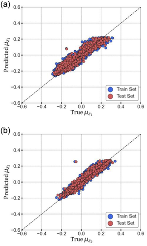
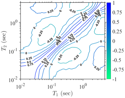
Hence, a 15-layered DNN with two nodes and linear activation function in the output layer is trained and used as the final method to estimate ${\mu _{{z_1}}}$ and ${\mu _{{z_2}}}$ using SC and IM_3s. The DNN is trained using a training dataset (randomly selected as 80% of the entire dataset), while evaluations are conducted on the remaining test dataset. The training is conducted using stochastic gradient descent with dropout and early stopping regularizations (Chollet, 2018). The true versus predicted ${\mu _{{z_1}}}$ and ${\mu _{{z_2}}}$ from the trained DNN are presented in Figure 8a,b, respectively. The nature of predictions is observed to be very close to the identity line (1:1) for both train and test sets, thereby indicating the good prediction power of the proposed DNN to estimate the two mean latent variables. The mean predictions of the trained DNN led to ${R^2}$ of 0.91 and 0.93 for ${\mu _{{z_1}}}$ and ${\mu _{{z_2}}}$ , respectively. A correlation coefficient of 0.91 was observed in DNN's predictions of ${\mu _{{z_1}}}$ and ${\mu _{{z_2}}}$ as compared to the true correlation coefficient of 0.88. This means the trained DNNs are highly successful in estimating ${\mu _{{z_1}}}$ and ${\mu _{{z_2}}}$ jointly. Due to the hierarchical nature of the data (i.e., multiple recordings from the same event and multiple recordings from different events), the residuals from the DNN–VAE framework are further used to conduct a mixed-effects regression (Demidenko, 2004) to develop inter-event ( ${\bm{\Phi }}$ ) and within-event ( ${\bm{T}}$ ) covariance matrices for the 96 periods. Since various available EEW systems compute different IMs for the incoming ground-motion and possess different site-characteristics, a separate DNN (which is usually less computationally expensive) allows the users to efficiently retrain the model to estimate the two latent variables as per their requirements.

4.3 Residual structure

Due to the hierarchical structure of the ground motions arising from multiple recordings from the same event and recordings from different events, the residuals between the

{{\bm{S}}_a}_{ij}

and predictions of DNN–VAE

{\widehat {{{\bm{S}}_a}}_{ij}}

are used to compute 96 values of inter-event and within-event variabilities for the ith event and jth recording. This is done by fitting a mixed-effects regression (Demidenko, 2004) model to the residuals as given in Equation (12) where

{\eta _i}

represents the between-event variability with

{\bm{T}}

variance matrix for 96 periods,

\ {\varepsilon _{ij}}

represents the within-event variability with

{\bm{\Phi }}

variance matrix for the 96 periods, and

{c_0}

represents any pending bias in the residuals for the 96 periods.

{c_0}

was observed to be very close to zero (failing the hypothesis test) and dropped in the overall analysis. Also, empirical Pearson correlations are computed for the residuals of the 96 periods (presented in Figure 9), which is then used to convert the inter-event and within-event variance matrices into their respective covariance matrices. In summary, the overall DNN–VAE framework is developed for mean predictions, and the residuals are used to construct between-event (

{\bm{\Phi }}

) and within-event (

{{\bf T}}

) covariance matrices.

\begin{equation}{{\bm{S}}_a}_{ij} - {\widehat {{{\bm{S}}_a}}_{ij}} = {c_0} + {\eta _i}\left( {0,{\bm{T}}} \right) + {\varepsilon _{ij}}\left( {0,{\bm{\Phi }}} \right)\end{equation}

(12)

5 IMPLEMENTATION OF ROSERS ON EXAMPLE SEISMIC EVENTS

The developed framework is exercised on three notable seismic events recorded in California (Ancheta, et al., 2014): (1) Northridge (M = 6.69, 1994); (2) Loma Prieta (M = 6.93, 1989); and (3) Whittier (M = 5.99, 1987). These events are considered pivotal points in the history of earthquake engineering as the reconnaissance data collected after these events led to substantial changes to the principles of structural analysis and design (Popov, et al., 1998). Apart from being historically significant seismic events, the three selected events were recorded at a relatively large number of stations, making them ideal candidates for validating the proposed ROSERS framework. Based on the criteria of ${R_{rup}} \le$ 90 km, NGA-West2 database contains recordings at (1) 137 stations for Northridge; (2) 79 stations for Loma Prieta; and (3) 108 stations for Whittier events. In this implementation example, the ROSERS framework is employed to conduct a seismic warning trigger classification for the selected three events. This means that for each event and station, decision analysis is performed based on whether the expected level of ${S_a}( T )$ (using the ROSERS framework) exceeds a hazard-consistent threshold ${S_{a,haz}}( T )$ for two natural periods, that is, 0.5 and 1.0 s. Due to the difference in the seismicity of each site, unlike other studies, this study does not utilize one strict ${S_a}( T )$ the threshold for all sites of the event. For example, a site close to an active seismic fault, ${S_a}( T )$ = 0.1 g may correspond to a frequent return period, and hence the structure/infrastructure of interest would not be highly susceptible to the resulting shaking. However, for a site away from active seismic faults, ${S_a}( T )$ = 0.1 g may represent a seismic event of significant hazard level and would lead to infrastructural devastation/disruption. Hence this study utilizes a hazard-consistent approach of trigger classification rather than a strict threshold. ${S_{a,haz}}( T )$ is determined for each station site by independently obtaining their respective ${S_a}( T )$ hazard curves using the US Geological Survey Unified Hazard Tool (2014; Petersen et al., 2020; developed by conducting probabilistic seismic hazard analysis [PSHA] for the target site) and computing ${S_a}( T )$ corresponding to six hazard levels, including mean return periods of 25, 50, 75, 100, 150, and 200 years. In simple terms, ${S_{a,haz}}( T )$ is the expected level of ${S_a}( T )$ for a given period and hazard level, which is obtained by considering all the known faults around the target site and performing a rigorous PSHA. Figure 10 presents the obtained ${S_{a,haz}}( T )$ (in units of g) against the ${R_{rup}}$ (in units of km) of their respective station sites for the three considered seismic events and two periods. As expected, for all the station sites, ${S_{a,haz}}( T )$ increases as the mean return period increases and for the same hazard level and site, ${S_{a,haz}}$ (T = 0.5 s; reaching up to ∼1.5 g) is greater than ${S_{a,haz}}$ (T = 1.0 s; reaching up to ∼1.2 g). It should be noted here that though the ${S_a}( T )$ for the selected events are expected to attenuate with an increase in ${R_{rup}}$ , ${S_{a,haz}}( T )$ remains unaffected as it represents the hazard-targeted ${S_a}( T )$ computed for each site representing its modeled seismicity (Field et al., 2009, 2014).

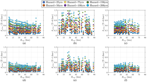
For the three seismic events, the ${S_{a,haz}}( T )$ values obtained for their respective station sites (for the six hazard levels and two periods) are used as thresholds to classify whether to trigger EEW warnings. For each event and station, the true ${S_a}( T )$ is known from the seismic recording and compared against their respective ${S_{a,haz}}( T )$ . If the true ${S_a}( T ) \ge {S_{a,haz}}( T )$ , then the seismic warning must be triggered (positive case) for the particular hazard level and period, while if ${S_a}( T ) < {S_{a,haz}}( T )$ no warning should be issued (negative case). For the selected events and stations, the initial 3 s of the seismic recordings are used in the proposed ROSERS framework to obtain ${S_a}( T )$ predictions and conduct trigger classification. The trigger classifications conducted using the ROSERS framework are compared against the true classification in two ways, using deterministic confusion matrices and probabilistic receiver operating characteristic (ROC) curves (Brown & Davis, 2006).

5.1 Trigger classification using confusion matrices

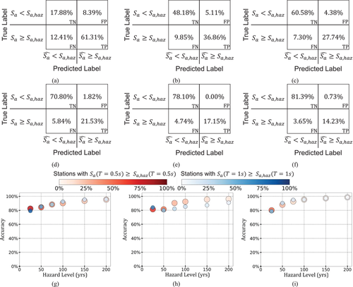
First, the mean predictions $\widehat {{S_a}( T )\ }$ are compared against ${S_{a,haz}}( T )$ as deterministic estimates to develop confusion matrices for each hazard level, event, and period. Figure 11a–f presents the confusion matrices generated for the Northridge event (consisting of 137 stations) for ${S_a}( {T = 1.0\ {\rm{s\ }}} )$ for the six hazard levels, where TN, FP, FN, and TP represent true negative, false positive, false negative, and true positive cases, respectively. In all cases, the percentages of TP and TN are significantly higher than FP and FN, which shows the high classification power of the proposed ROSERS framework. As observed in Figure 10, ${S_{a,haz}}( T )$ increases with the increase in hazard level, which leads to a lower number of stations with true ${S_a}( T ) \ge {S_{a,haz}}( T )$ . Hence, in Figure 11e,f, it can be observed that the percentage of TP and FN cases are lower than those in Figure 11a–d. However, in general, it can be observed that TP and TN are significantly higher than FP and FN, thereby demonstrating the high classification accuracy of ROSERS. Similar confusion matrices were developed and analyzed for all other cases. To summarize the results, the accuracies (i.e., $( {{\rm{TP}} + {\rm{TN}}} )/( {{\rm{TP}} + {\rm{TN}} + {\rm{FP}} + {\rm{FN}}} )$ ) for the six hazard levels and two periods are presented in Figure 11g,h,i for the Northridge, Loma Prieta, and Whittier events, respectively. In these figures, the color shade of the markers represents the percentage of stations with true ${S_a}( T ) \ge {S_{a,haz}}( T )$ (i.e., FN + TP). It can be observed in Figure 11g–i that, with an increase in hazard level, the accuracy of classification increases from ∼80% to ∼99% for both periods and three seismic events. This means that the proposed framework is capable of accurately estimating whether ${S_a}( T ) \ge {S_{a,haz}}( T )$ and conduct trigger classification for low-rise (∼T = 0.5 s) as well as mid-rise (∼T = 1 s) structures. Furthermore, as mentioned earlier, it can be observed from all cases that, with an increase in hazard level, the color shades of the scatter plots tend to fade, indicating that a lower number of stations lead to true ${S_a}( T ) \ge {S_{a,haz}}( T )$ . This indicates that the shaking observed at the stations for their respective earthquake events is generally lower than the expected shaking computed through PSHA of the region/sites for higher hazard levels. Due to this, a lower number of TP cases and a more significant number of TNs are noticed for the increased hazard levels for all three events. However, the framework is continuously observed to lead to higher accuracies with a more significant number of TNs and a smaller number of FPs. Consequently, the proposed framework can help in decreasing the number of false alarms, thereby reducing the nuisance and hindrance caused to a community. In general, the results indicate that the framework's accuracy for all events and periods is above ∼80% and tends to increase for shaking levels with longer return periods (higher hazard levels), leading up to ∼99% for a 200-year return period. Given that the predictions of the proposed framework are tested against hazard-consistent levels of ${S_a}( T )$ (unlike previous studies such as Münchmeyer et al. (2020), Caruso et al. (2017), Colombelli & Zollo (2015), Hsu et al. (2013); that use a constant ${S_a}( T )$ level for testing), the classification results are observed to be on the high end of accuracy.

5.2 Trigger classification using ROC-AUC curves

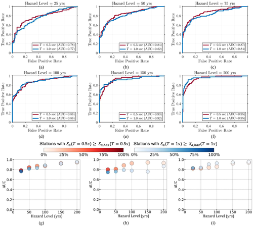
In the second set of comparisons, the mean predictions $\widehat {{S_a}( T )\ }$ are combined with their inter-event and within-event variabilities of the residuals to construct a probabilistic distribution of the predictions for the particular period. The probabilistic distributions are used to obtain $P( {\widehat {{S_a}( T )} \ge {S_{a,haz}}( T )} )$ for all three events, six hazard levels, and two natural periods, which are compared against the true classification of ${S_a}( T ) \ge {S_{a,haz}}( T )$ using the ROC curves. The area under the ROC curve is termed Area Under Curve (AUC), representing the degree or measure of separability between TP and FP rates for various thresholds. The ROC-AUC curves for the six hazard levels for ${S_a}( {T = 1.0\ {\rm{s}}} )$ for the Northridge event are presented in Figure 12a–f; the AUC scores of the cases are shown in Figure 12g–i for the three events and two periods. Similar to the observation made in terms of prediction accuracies, AUC values are observed to be higher than ∼0.8 for all cases and tend to increase with an increase in hazard levels. The ROC curves in Figure 12a–f show how the ROSERS framework's distinguishing power between the two classes improves for ${S_a}( T )$ with a higher hazard level (i.e., more critical) leading up to AUC = 0.95 for a 200-year return period. This further highlights the accuracy of the decision-making power of the proposed framework to issue probabilistic warnings during a seismic event, especially for more dangerous shaking levels (higher return periods).

6 CONCLUSIONS

This study introduced a deep learning-based on-site EEW framework named. The framework utilizes a pre-trained DNN to estimate two mean latent variables (that represent statistical surrogates of the ${S_a}( T )$ spectrum) using the SC and initial 3 s of on-site ground-motion after p-wave detection. The initial 3 s of the on-site ground-motion waveform are used to compute seven IMs representing the energy, amplitude, significant duration, and frequency content of the initial seconds (mainly p-waves) of the 3 s of the arriving ground-motion waveform. The computed IMs are combined with two site- parameters and used as inputs to a trained DNN that estimates two mean latent variables that are used in a trained decoder of VAE to estimate ${\rm{PGA}}$ and 95-period spectral acceleration ( ${S_a}( T )$ ) response spectrum of the expected on-site ground-motion.

The trained framework performs well on the used dataset and leads to high prediction power. The prediction of the complete ${S_a}( T )$ spectrum (while inherently maintaining the cross-correlations) with only 3 s of the initial ground-motion waveform in a highly accurate manner (coupled with an average prediction time of less than 1 s) makes the proposed framework valuable for real-time EEW decision-making and near-real-time rapid response systems.

The proposed ROSERS framework was first trained and tested on the NGA-West2 database and then exercised on over 300 recording stations of three historical seismic events recorded in California. The expectation for EEW is that if ${S_a}( T ) > {S_{a,haz}}( T )$ for the target site, then the alarm must be triggered. For the three events, the true recorded ${S_a}( T )$ and ${S_{a,haz}}( T )$ is available; hence, the true labels and thresholds are known. Using the first 3 s (after detection of p-waves) of the available recordings, the ROSERS framework was implemented for all stations of the three events for two hazard levels and periods. The outputs of the ROSERS framework were analyzed using confusion matrices and ROC curves. Results of the confusion matrices show that the ROSERS framework leads to high accuracy (> 80%) in most cases of the decision classification. Furthermore, the framework leads to 0.8 <AUC < 0.95 demonstrating excellent classification power even for the infrequent earthquake events.

The framework developed in this study can help improve existing on-site EEW approaches. While the analysis presented in this paper demonstrate that the framework has good prediction power to accurately estimate the ${S_a}( T )$ spectrum using the initial 3 s of the ground motions, future analyses should extend the reliability and confidence in the proposed framework, particularly in actual real-time settings. Currently, the framework is mainly trained using a database of processed crustal ground motions. Testing it on unprocessed datasets can be valuable for validation in a real-time setting. However, the framework's performance is not expected to significantly change within this backdrop as the data-driven nature of the framework would adapt to any discrepancies due to the addition of station noise in the considered few seconds of early p-waves. Furthermore, the framework can be extended to regional EEW systems by utilizing the spatially correlated prior estimates of the latent variables at stations farther from the source. In addition, similar to GMMs, the proposed framework can be trained independently for different geographic regions to obtain their localized latent spaces and DNN structures. This can also accelerate the understanding of regional seismicity from a mathematical perspective.

Finally, the developed framework can be tested by conducting a consequential analysis on the false positives and false negatives cases to make end-users and stakeholders aware of the significances of various decisions. In general, as quoted by J. R. Tolkien, “False hopes are more dangerous than fears,”—It is believed that false negatives are riskier than false positives; however, the case is not so evident in earthquakes as even false positives can lead to significant economic losses for downtime, shutdowns, and panic. Furthermore, a community may also face psychological hindrances to return to work after a false alarm. However, on the flip side, false positives can also be beneficial in some ways, such as conducting unplanned drills for seismic events, checks for preparedness, and so forth (Velazquez et al., 2020).

DATA AND RESOURCE AVAILABILITY

The recorded ground motions used in this study can be obtained from NGAWest2 database (https://ngawest2.berkeley.edu/). The authors have also developed an executable software to utilize the proposed ROSERS framework. The software can be download from the GitHub repository (https://github.com/jfayaz/ROSERS).

ACKNOWLEDGMENTS

This research is funded by the European Union's Horizon 2020 research and innovation program, specifically Grant Agreement Number 821046: TURNkey “Towards more Earthquake-resilient Urban Societies through a Multi-sensor-based Information System enabling Earthquake Forecasting, Early Warning and Rapid Response actions.”

REFERENCES

Akazawa, T. (2004). A technique for automatic detection of onset time of P- and S-phases in strong motion records. 13th World Conference on Earthquake Engineering, Vancouver, British Columbia, Canada.
Google Scholar
Ancheta, T. D., Darragh, R. B., Stewart, J. P., Seyhan, E., Silva, W. J., Chiou, B. S. J., Wooddell, K. E., Graves, R. W., Kottke, A. R., Boore, D. M., Kishida, T., Donahue, J. L. (2014). PEER NGA-West2 database. Earthquake Spectra, 30(3), 989–1005.
10.1193/070913EQS197M
Web of Science® Google Scholar
Anon. (2011). IEEE standard for transitions, pulses, and related waveforms. Waveform Generation, Measurement, and Analysis Committee IEEE Instrumentation and Measurement Society. https://doi.org/10.1109/IEEESTD.2011.6016198
10.1109/IEEESTD.2011.6016198
Google Scholar
Bazzurro, P., Cornell, C. A., Shome, N., & Carballo, J. E. (1998). Three proposals for characterizing MDOF nonlinear seismic response. Journal of Structural Engineering, 124(11), 1281–1289. https://doi.org/10.1061/(asce)0733-9445(1998)124:11(1281)
10.1061/(asce)0733?9445(1998)124:11(1281)
Web of Science® Google Scholar
Bhardwaj, R., Sharma, M. L., & Kumar, A. (2016). Multi-parameter algorithm for earthquake early warning. Geomatics, Natural Hazards and Risk, 7(4), 1242–1264. https://doi.org/10.1080/19475705.2015.1069409
10.1080/19475705.2015.1069409
Web of Science® Google Scholar
Blei, D. M., Kucukelbir, A., & McAuliffe, J. D. (2017). Variational inference: A review for statisticians. Journal of the American Statistical Association, 112(518), 859–877. https://doi.org/10.1080/01621459.2017.1285773
10.1080/01621459.2017.1285773
CAS Web of Science® Google Scholar
Boore, D. M., & Bommer, J. J. (2005). Processing of strong-motion accelerograms: Needs, options and consequences. Soil Dynamics and Earthquake Engineering, 25(2), 93–115. https://doi.org/10.1016/j.soildyn.2004.10.007
10.1016/j.soildyn.2004.10.007
Web of Science® Google Scholar
Borodinov, N., Neumayer, S., Kalinin, S. V., Ovchinnikova, O. S., Vasudevan, R. K., & Jesse, S. (2019). Deep neural networks for understanding noisy data applied to physical property extraction in scanning probe microscopy. npj Computational Materials, 5(1), 1–8. https://doi.org/10.1038/s41524-019-0148-5
10.1038/s41524?019?0148?5
Web of Science® Google Scholar
Brondi, P., Picozzi, M., Emolo, A., Zollo, A., & Mucciarelli, M. (2015). Predicting the macroseismic intensity from early radiated P wave energy for on-site earthquake early warning in Italy. Journal of Geophysical Research: Solid Earth, 120(10), 7174–7189. https://doi.org/10.1002/2015JB012367
10.1002/2015JB012367
Web of Science® Google Scholar
Brown, C. D., & Davis, H. T. (2006). Receiver operating characteristics curves and related decision measures: A tutorial. Chemometrics and Intelligent Laboratory Systems, 80(1), 24–38. https://doi.org/10.1016/j.chemolab.2005.05.004
10.1016/j.chemolab.2005.05.004
CAS Web of Science® Google Scholar
Caruso, A., Colombelli, S., Elia, L., Picozzi, M., & Zollo, A. (2017). An on-site alert level early warning system for Italy. Journal of Geophysical Research: Solid Earth, 122(3), 2106–2118. https://doi.org/10.1002/2016JB013403
10.1002/2016JB013403
Web of Science® Google Scholar
Chen, T., & Guestrin, C. (2016). XGBoost. Proceedings of the 22nd ACM SIGKDD International Conference on Knowledge Discovery and Data Mining, San Francisco, CA.
Google Scholar
Chollet, F. (2018). Deep learning with Python. Manning Publications.
Google Scholar
Colombelli, S., & Zollo, A. (2015). Fast determination of earthquake magnitude and fault extent from real-time P -wave recordings. Geophysical Journal International, 202(2), 1158–1163. https://doi.org/10.1093/gji/ggv217
10.1093/gji/ggv217
Web of Science® Google Scholar
Cortes, C., Vapnik, V., & Saitta, L. (1995). Support-vector networks editor (Vol., 20). Kluwer Academic Publishers.
Google Scholar
Cremen, G., & Galasso, C. (2020). Earthquake early warning: Recent advances and perspectives. Earth-Science Reviews, 205, 103184.
10.1016/j.earscirev.2020.103184
Web of Science® Google Scholar
Cremen, G., & Galasso, C. (2021). A decision-making methodology for risk-informed earthquake early warning. Computer-Aided Civil and Infrastructure Engineering, 36(6), 747–761. https://doi.org/10.1111/mice.12670
10.1111/mice.12670
Web of Science® Google Scholar
Demidenko, E. (2004). Mixed models. John Wiley & Sons, Inc.
10.1002/0471728438
Google Scholar
Fayaz, J., Medalla, M., & Zareian, F. (2020). Sensitivity of the response of box-girder seat-type bridges to the duration of ground motions arising from crustal and subduction earthquakes. Engineering Structures, 219, 110845. https://doi.org/10.1016/j.engstruct.2020.110845
10.1016/j.engstruct.2020.110845
Web of Science® Google Scholar
Fayaz, J., Xiang, Y., & Zareian, F. (2021). Generalized ground motion prediction model using hybrid recurrent neural network. Earthquake Engineering and Structural Dynamics, 50(6), 1539–1561. https://doi.org/10.1002/eqe.3410
10.1002/eqe.3410
Web of Science® Google Scholar
Field, E. H., Arrowsmith, R. J., Biasi, G. P., Bird, P., Dawson, T. E., Felzer, K. R., Jackson, D. D., Johnson, K. M., Jordan, T. H., Madden, C., Michael, A. J., Milner, K. R., Page, M. T., Parsons, T., Powers, P. M., Shaw, B. E., Thatcher, W. R., Weldon, R. J., & Zeng, Y. (2014). Uniform california earthquake rupture forecast, Version 3 (UCERF3)–The time-independent model. Bulletin of the Seismological Society of America, 104(3), 1122. https://doi.org/10.1785/0120130164
10.1785/0120130164
Web of Science® Google Scholar
Field, E. H., Dawson, T. E., Felzer, K. R., Frankel, A. D., Gupta, V., Jordan, T. H., Parsons, T., Petersen, M. D., Stein, R. S., Weldon, R. J., & Wills, C. J. (2009). Uniform California earthquake rupture forecast, Version 2 (UCERF 2). Bulletin of the Seismological Society of America, 99(4), 2053–2107. https://doi.org/10.1785/0120080049
10.1785/0120080049
Web of Science® Google Scholar
Freedman, D. A. (2009). Statistical models. Cambridge University Press.
Google Scholar
Gorijala, M., & Dukkipati, A. (2017). Image generation and editing with variational info generative Adversarial Networks. arXiv preprint arXiv:1701.04568.
Google Scholar
Gustafson, S. C., Little, G. R., & Simon, G. M. (1990). Neural network for interpolation and extrapolation. In S. K. Rogers (Ed.), Applications of artificial neural networks (Vol., 1294, pp. 389–95). SPIE.
Google Scholar
Hoshiba, M., & Aoki, S. (2015). Numerical shake prediction for earthquake early warning: data assimilation, real-time shake mapping, and simulation of wave propagation. Bulletin of the Seismological Society of America, 105(3), 1324–1338. https://doi.org/10.1785/0120140280
10.1785/0120140280
Web of Science® Google Scholar
Hsu, T. Y.,Wu, R. T., & Chang, K. C. (2016). Two novel approaches to reduce false alarm due to non-earthquake events for on-site earthquake early warning system. Computer-Aided Civil and Infrastructure Engineering, 31(7), 535–549.
10.1111/mice.12191
Web of Science® Google Scholar
Hsu, T. Y, Huang, S. K., Chang, Y W., Kuo, C. H., Lin, C. M., Chang, T. M., Wen, K. L., & Loh, C. H. (2013). Rapid on-site peak ground acceleration estimation based on support vector regression and P-wave features in Taiwan. Soil Dynamics and Earthquake Engineering, 49, 210–217. https://doi.org/10.1016/j.soildyn.2013.03.001
10.1016/j.soildyn.2013.03.001
Web of Science® Google Scholar
Iaccarino, A. G., Picozzi, M., Bindi, D., & Spallarossa, D., (2020). On-site earthquake early warning: Predictive models for acceleration response spectra considering site effects. Bulletin of the Seismological Society of America, 110, 1289–1304
Web of Science® Google Scholar
Iervolino, I., Giorgio, M., Galasso, C., & Manfredi, G. (2009). Uncertainty in early warning predictions of engineering ground motion parameters: What really matters? Geophysical Research Letters, 36(5), L00B06. https://doi.org/10.1029/2008GL036644
10.1029/2008GL036644
Web of Science® Google Scholar
Jozinović, D., Lomax, A., Štajduhar, I., & Michelini, A., (2020). Rapid prediction of earthquake ground shaking intensity using raw waveform data and a convolutional neural network. Geophysical Journal International, 222, 1379–1389.
10.1093/gji/ggaa233
Web of Science® Google Scholar
Jumper, J., Evans, R., Pritzel, A., Green, T., Figurnov, M., Ronneberger, O., Tunyasuvunakool, K., Bates, R., Žídek, A., Potapenko, A., Bridgland, A., Meyer, C., Kohl, S. A. A., Ballard, A. J., Cowie, A., Romera-Paredes, B., Nikolov, S., Jain, R., Adler, J., … Hassabis, D. (2021). Highly accurate protein structure prediction with AlphaFold. Nature, 596(7873), 583–589. https://doi.org/10.1038/s41586-021-03819-2
10.1038/s41586-021-03819-2
CAS PubMed Web of Science® Google Scholar
Kalkan, E. (2016). An automatic p-phase arrival-time picker. Bulletin of the Seismological Society of America, 106(3), 971–986. https://doi.org/10.1785/0120150111.
10.1785/0120150111
Web of Science® Google Scholar
Kingma, D. P., & Ba, J. (2014). Adam: A method for stochastic optimization. 3rd International Conference on Learning Representations, ICLR 2015, San Diego, CA.
Google Scholar
Kingma, D. P., & Welling, M. (2019). An introduction to variational autoencoders. Foundations and Trends in Machine Learning, 12(4), 307–392.
10.1561/2200000056
Web of Science® Google Scholar
Kramer. (1995). Geotechnical earthquake engineering (1st ed.). Pearson.
Google Scholar
Kullback, S., & Leibler, R. A. (1951). On information and sufficiency. The Annals of Mathematical Statistics, 22(1), 79–86. https://doi.org/10.1214/aoms/1177729694
10.1214/aoms/1177729694
Web of Science® Google Scholar
LemaˆıtreLemaˆıtre, G., Nogueira, F., & Aridas Char, C. K. (2017). Imbalanced-learn: A Python toolbox to tackle the curse of imbalanced datasets in machine learning. Journal of Machine Learning Research, 18, 1–5.
Web of Science® Google Scholar
Li, H., Yi, W. J., & Yuan, X. X. (2013). Fuzzy-valued intensity measures for near fault pulse-like ground motions. Computer Aided Civil and Infrastructure Engineering, 28(10), 780–795.
10.1111/mice.12053
CAS Web of Science® Google Scholar
Meier, M. A. (2017). How ‘Good’ are real-time ground motion predictions from earthquake early warning systems? Journal of Geophysical Research: Solid Earth, 122(7), 5561–5577. https://doi.org/10.1002/2017JB014025.
10.1002/2017JB014025
Web of Science® Google Scholar
Minson, S. E., Baltay, A. S., Cochran, E. S., Hanks, T. C., Page, M. T., McBride, S. K., Milner, K. R., & Meier, M. A. (2019). The limits of earthquake early warning accuracy and best alerting strategy. Scientific Reports, 9(1), 1–13. https://doi.org/10.1038/s41598-019-39384-y.
10.1038/s41598?019?39384?y
CAS PubMed Web of Science® Google Scholar
Mu, H. Q., & Yuen, K. V. (2016). Ground motion prediction equation development by heterogeneous Bayesian learning. Computer-Aided Civil and Infrastructure Engineering, 31, 761–776.
10.1111/mice.12215
Web of Science® Google Scholar
Münchmeyer, J., Bindi, D., Leser, U., & Tilmann, F. (2020). The transformer earthquake alerting model: A new versatile approach to earthquake early warning. Geophysical Journal International, 225(1), 646–656. https://doi.org/10.1093/gji/ggaa609
10.1093/gji/ggaa609
Web of Science® Google Scholar
Panakkat, A., & Adeli, H., (2008). Recent efforts in earthquake prediction (1990–2007). Natural Hazards Review, 9(2), 70–80.
10.1061/(ASCE)1527-6988(2008)9:2(70)
Google Scholar
Panakkat, A., & Adeli, H., (2009). Recurrent neural network for approximate earthquake time and location prediction using multiple seismicity indicators. Computer-Aided Civil and Infrastructure Engineering, 24(4), 280–292.
10.1111/j.1467-8667.2009.00595.x
Web of Science® Google Scholar
Petersen, M. D., Shumway, A. M., Powers, P. M., Mueller, C. S., Moschetti, M. P., Frankel, A. D., Rezaeian, S., McNamara, D. E., Luco, N., Boyd, O. S., Rukstales, K. S., Jaiswal, K. S., Thompson, E. M., Hoover, S. M., Clayton, B. S., Field, E. H., & Zeng, Y. (2020). The 2018 update of the U.S. National Seismic Hazard Model: Overview of model and implications. Earthquake Spectra, 36(1), 5–41. https://doi.org/10.1177/8755293019878199
10.1177/8755293019878199
Web of Science® Google Scholar
Popov, P., Egor, T. Shuoh, Y., & Chang, S. P. (1998). Design of steel MRF connections before and after 1994 Northridge earthquake. Engineering Structures, 20(12), 1030–1038. https://doi.org/10.1016/S0141-0296(97)00200-9
10.1016/S0141-0296(97)00200-9
Web of Science® Google Scholar
Rafiei, M., & Adeli, H., (2017). NEEWS: A novel earthquake early warning model using neural dynamic classification and neural dynamic optimization. Soil Dynamics and Earthquake Engineering, 100, 417–427.
10.1016/j.soildyn.2017.05.013
Web of Science® Google Scholar
Rosenblatt, F. (1958). The perceptron: A probabilistic model for information storage and organization in the brain. Psychological Review, 65(6), 386–408. https://doi.org/10.1037/h0042519
10.1037/h0042519
CAS PubMed Web of Science® Google Scholar
Sleeman, R., & van Eck, T. (1999). Robust automatic P-Phase picking: An on-line implementation in the analysis of broadband seismogram recordings. Physics of the Earth and Planetary Interiors, 113(1–4). https://doi.org/10.1016/S0031-9201(99)00007-2
10.1016/S0031?9201(99)00007?2
Web of Science® Google Scholar
Solomon, O. M., Larson, D. R., & Paulter, N. G. (2001). Comparison of some algorithms to estimate the low and high state level of pulses." IMTC 2001. Proceedings of the 18th IEEE Instrumentation and Measurement Technology Conference. Rediscovering Measurement in the Age of Informatics (Cat. No.01CH 37188), Budapest, Hungary (pp. 96–101). https://doi.org/10.1109/IMTC.2001.928794
10.1109/IMTC.2001.928794
Google Scholar
U.S. Geological Survey (USGS) (2019). Unified Hazard Tool (dynamic conterminous US 2014 edition). https://earthquake.usgs.gov/hazards/interactive/index.php
Google Scholar
Vamvatsikos, D., & Cornell, C. A. (2002). Incremental dynamic analysis. Earthquake Engineering and Structural Dynamics, 31(3), 491–514. https://doi.org/10.1002/eqe.141
10.1002/eqe.141
Web of Science® Google Scholar
Velazquez, O., Pescaroli, G., Cremen, G., & Galasso, C. (2020). A review of the technical and socio-organizational components of earthquake early warning systems. Frontiers in Earth Science, 8(October), 1–19. https://doi.org/10.3389/feart.2020.533498.
10.3389/feart.2020.533498
Web of Science® Google Scholar
Wald, D. J. (2020). Practical limitations of earthquake early warning. Earthquake Spectra, 36(3), 1412–1447. https://doi.org/10.1177/8755293020911388
10.1177/8755293020911388
Web of Science® Google Scholar
Wu, S., Beck, J. L., & Heaton, T. H. (2013). ePAD: Earthquake probability-based automated decision-making framework for earthquake early warning. Computer-Aided Civil and Infrastructure Engineering, 28, 737–752.
10.1111/mice.12048
Web of Science® Google Scholar
Wu, Y. -M., & Kanamori, H. (2008). Development of an earthquake early warning system using real-time strong motion signals. Sensors, 8(1), 1–9. https://doi.org/10.3390/s8010001
10.3390/s8010001
Web of Science® Google Scholar
Xu, K., Zhang, M., Li, J., Du, S. S., Kawarabayashi, K. -I., & Jegelka, S. (2021). How neural networks extrapolate: From feedforward to graph neural networks. International Conference on Learning Representations, Vienna, Austria.
Google Scholar
Zarrin, M., Abyani, M., & Asgarian, B. (2020). A statistical study on lognormal central tendency estimation in probabilistic seismic assessments. Structure and Infrastructure Engineering, 16(5), 803–819. https://doi.org/10.1080/15732479.2019.1668813
10.1080/15732479.2019.1668813
Web of Science® Google Scholar

Citing Literature

Volume38, Issue1

1 January 2023

Pages 87-103

A deep neural network framework for real-time on-site estimation of acceleration response spectra of seismic ground motions

Abstract

1 INTRODUCTION

2 PROPOSED FRAMEWORK