Mixed ancestry from wild and domestic lineages contributes to the rapid expansion of invasive feral swine
Abstract
Invasive alien species are a significant threat to both economic and ecological systems. Identifying the processes that give rise to invasive populations is essential for implementing effective control strategies. We conducted an ancestry analysis of invasive feral swine (Sus scrofa, Linnaeus, 1758), a highly destructive ungulate that is widely distributed throughout the contiguous United States, to describe introduction pathways, sources of newly emergent populations and processes contributing to an ongoing invasion. Comparisons of high-density single nucleotide polymorphism genotypes for 6,566 invasive feral swine to a comprehensive reference set of S. scrofa revealed that the vast majority of feral swine were of mixed ancestry, with dominant genetic associations to Western heritage breeds of domestic pig and European populations of wild boar. Further, the rapid expansion of invasive feral swine over the past 30 years was attributable to secondary introductions from established populations of admixed ancestry as opposed to direct introductions of domestic breeds or wild boar. Spatially widespread genetic associations of invasive feral swine to European wild boar deviated strongly from historical S. scrofa introduction pressure, which was largely restricted to domestic pigs with infrequent, localized wild boar releases. The deviation between historical introduction pressure and contemporary genetic ancestry suggests wild boar-hybridization may contribute to differential fitness in the environment and heightened invasive potential for individuals of admixed domestic pig–wild boar ancestry.
1 INTRODUCTION
With increasing globalization, invasive alien species (IAS) have emerged as a significant and growing threat to both economic and ecological systems. Numerous studies have quantified the costs of IAS to specific economic sectors such as agriculture, silviculture and tourism (Anderson, Slootmaker, Harper, Holderieath, & Shwiff, 2016; Charles & Dukes, 2008; Eiswerth, Darden, Johnson, Agapoff, & Harris, 2005; Holmes, Aukema, Von Holle, Liebhold, & Sills, 2009). However, the full costs of IAS are difficult to monetize due to their impacts on ecosystem services, the aesthetic and cultural value of landscapes, and human health and well-being (Pejchar & Mooney, 2009). Furthermore, IAS pose a significant threat to biodiversity by negatively impacting native species through predation and competition (Human & Gordon, 1996; Leighton, Horrocks, & Kramer, 2011; Lowe, Browne, Boudjelas, & De Poorter, 2000; Wilcove, Rothstein, Dubow, Phillips, & Losos, 1998; Wiles, Bart, Beck, & Aguon, 2003). In extreme cases IAS can completely reconfigure ecosystems through the exclusion of foundation species, alteration of disturbance regimes, displacement of entire native communities or formation of alien monocultures (Balch, Bradley, D'Antonio, & Gomez-Dans, 2013; Bankovich, Boughton, Boughton, Avery, & Wisely, 2016; Ellison et al., 2005; Hutchinson & Vankat, 1997; Tabak, Poncet, Passfield, Goheen, & Del Rio, 2016; Wiles et al., 2003). In the United States (US), as many as 87% of imperiled species are directly threatened by IAS (McClure, Burdett, Farnsworth, Sweeney, & Miller, 2018).
Identifying the processes by which IAS are introduced is essential for implementing effective policies, quarantine procedures, or other strategies to control ongoing invasions or prevent future invasions (Estoup & Guillemaud, 2010; Lawson Handley et al., 2011; Lombaert et al., 2010; Willson, Dorcas, & Snow, 2011). Traditionally, inferring processes contributing to the establishment of invasive populations has depended on direct observations or historical accounts, which reconstruct patterns of human travel and trade to identify potential invasion pathways (Estoup & Guillemaud, 2010). More recently, the application of genetic tools to study IAS has elucidated many aspects of the invasion process (Lawson Handley et al., 2011). By comparing genetic attributes of IAS populations with potential sources, ecological genetic methods may corroborate observations or reveal cryptic processes leading to invasion that may not have been recognized from the historical record (Estoup & Guillemaud, 2010; Lawson Handley et al., 2011; Lombaert et al., 2010; Willson et al., 2011).
Following initial introduction of IAS, genetic processes may have a direct impact on subsequent demographic rates and dictate whether propagules fail to establish or become highly invasive (Bock et al., 2015; Lawson Handley et al., 2011). For example, as a consequence of founder effects, the ability of an introduced population to adapt to novel environmental conditions may be constrained by low genetic diversity and concomitant low evolutionary potential (Estoup et al., 2016). However, when populations of IAS arise through contributions from multiple sources, genetic diversity may be enriched beyond that commonly found within populations in the native range, increasing the likelihood of successful establishment (Kolbe et al., 2004; Lavergne & Molofsky, 2007). Furthermore, the admixture of individuals from disparate source populations may result in the emergence of novel phenotypes through the alignment and integration of phenotypic traits that are characteristic of the distinct contributing lineages, potentially eliciting an evolutionary shift that may increase fitness and allow an introduced population to become highly invasive (Bossdorf et al., 2005; Facon et al., 2006; Lavergne & Molofsky, 2007; Lombaert et al., 2010; van Boheemen et al., 2017).
It is within the evolutionary context of biological invasions that we applied the tools of ecological genetics to gain an understanding of the genetic ancestry and introduction processes that have led to the establishment and rapid expansion of invasive feral swine (Sus scrofa, Linnaeus, 1758) throughout much of the contiguous US. Hereafter, we use the term “invasive feral swine” to refer to free-living members of S. scrofa sampled throughout the invaded range in the contiguous US and to differentiate such individuals from domestic pigs maintained in captive herds or wild boar sampled throughout their native range in Eurasia, which were also included in this analysis. Invasive feral swine in the contiguous US date back to 1539, stemming from the introduction of domestic pigs by Spanish explorers (Mayer & Brisbin, 1991; Zadik, 2000). Initial populations were subsequently augmented by free-range pig husbandry, specifically the seasonal release of pigs into forested habitats to fatten on mast crops, which was a common practice in the US until the mid-1900s (Mayer & Brisbin, 1991). With growing interest in recreational hunting through the late 1800s and early 1900s, wild boar were imported to the US from Europe and introduced into established invasive feral swine populations to improve the phenotypic appearance and hunting appeal of this species (Mayer & Brisbin, 1991). Despite a long history of invasive feral swine in the contiguous US, populations were largely restricted to localized areas in the southeastern US, Texas and California up to 1988 (Figure 1; Bevins, Pedersen, Lutman, Gidlewski, & Deliberto, 2014; Nolte & Anderson, 2015). However, since 1988 there has been a marked and accelerating increase in the distribution of feral swine, with populations expanding from 17 states in 1988 to 34 states in 2016 (McClure et al., 2015; Nolte & Anderson, 2015; Snow, Jarzyna, & VerCauteren, 2017) and a corresponding 2.8-fold increase in estimated abundance (from ~2.5 to 6.9 million; Lewis et al., 2019).

To identify the genetic origins and introduction processes contributing to this ongoing invasion, we characterized the genetic ancestry of invasive feral swine by comparing high-density (HD) single nucleotide polymorphism (SNP) genotypes for 6,566 feral swine sampled throughout the invaded range within the contiguous US to a comprehensive reference set for S. scrofa—consisting of commercial and heritage domestic pig breeds, wild boar populations sampled throughout their native range and sister species. Furthermore, we evaluated whether the recent expansion of invasive feral swine could be attributed to the growth of previously established invasive populations or represented the effect of sustained propagule pressure (sensu Simberloff, 2009) associated with novel introductions from distinct genetic lineages (i.e., domestic breeds, wild boar or companion animals).
2 MATERIALS AND METHODS
2.1 Invasive feral swine sample collection and genotyping
Feral swine samples were collected throughout the entirety of the invaded range within the contiguous US as an extension of damage mitigation efforts led by the United States Department of Agriculture (USDA; Figure 1). Specifically, samples were collected by USDA-Wildlife Services personnel from invasive feral swine that were lethally removed through trapping or targeted sharpshooting, with the management objective of reducing threats to agriculture, natural resources, and the health of humans and livestock. Given that samples were collected through agency control efforts, sampling probably had less sex, age or phenotypic bias than would be expected if samples had been collected opportunistically through hunter submissions. Samples were collected from 2 June 2001 to 9 August 2017 with the majority (89%) of samples collected since 2014 (median collection date = 14 December 2015; Appendix S1). The increase in sample collection over recent years (2014–2017) reflects the establishment of the National Feral Swine Damage Management Program—a USDA programme to facilitate feral swine control efforts throughout the invaded range and collection of associated biological samples. Prior to 2014, samples were collected by USDA during disease surveillance efforts or from feral swine that were otherwise culled in response to local management needs. Given that genetic samples were acquired ancillary to legally authorized control of invasive feral swine, sample collection was exempted from Institutional Animal Care and Use Committee review.
We extracted invasive feral swine DNA from various biological sample types (hair, pinna and kidney) using multiple commercially available extraction kits (MagMax DNA, Thermo Fisher Scientific; DNeasy Blood and Tissue and QIAamp DNA Investigator, Qiagen). Invasive feral swine were genotyped using Illumina BeadChip microarrays developed for pigs (PorcineSNP60 version 2, n = 168; Genomic Profiler for Porcine HD, n = 6,398, exclusively licensed to GeneSeek, a Neogen Corporation; Ramos et al., 2009). Combining genotypes produced across multiple Illumina BeadChips microarrays yielded 29,375 common autosomal loci, with all available loci retained for subsequent analyses. Based upon the available loci, we removed samples with call rates <95%, thus retaining 6,566 invasive feral swine for analysis.
2.2 Sus scrofa reference set assembly
We assembled our reference set by compiling domestic pig and native wild boar HD SNP genotypes from previously published data sets (n = 2,450; Alexandri et al., 2017; Burgos-Paz et al., 2013; Goedbloed, Megens, et al., 2013; Iacolina et al., 2016; Roberts & Lamberson, 2015; Yang et al., 2017), which we augmented with novel genotypes produced by our research group (n = 566; produced with extraction methods described above and genotyped with the Genomic Profiler for Porcine HD [GeneSeek]). To align with feral swine genotypes, we restricted our reference set to data sets similarly produced with either the PorcineSNP60 (versions 1 and 2; Illumina) or Genomic Profiler for Porcine HD (GeneSeek) BeadChip microarrays (Ramos et al., 2009). In total, we compiled 3,016 reference samples that represented 132 distinct reference groups (105 domestic pig breeds, 23 native wild boar populations and four sister taxa; Table 1). Hereafter, we use the term “reference group” to denote groups of reference samples organized by breed for domestic pigs or country of origin for native wild boar, and “reference set” to refer to the collection of all reference samples.
| Reference group | n | Reference cluster | Reference type |
|---|---|---|---|
| Berkshire | 80 | K1 | Domestic pig |
| Hampshire | 68 | K2 | Domestic pig |
| Sus verrucosus | 10 | K3 | Sister taxa |
| Phacochoerus africanus | 8 | K3 | Sister taxa |
| Sus celebensis | 6 | K3 | Sister taxa |
| Babyrousa babyrussa | 4 | K3 | Sister taxa |
| Wild boar_Sardinia | 92 | K4 | Native wild boar |
| British Saddleback | 25 | K5 | Domestic pig |
| Pietrain | 66 | K6 | Domestic pig |
| Chester White | 26 | K7 | Domestic pig |
| Middle White | 19 | K7 | Domestic pig |
| Chato Murciano | 18 | K7 | Domestic pig |
| White Steppe | 16 | K7 | Domestic pig |
| Breitov | 13 | K7 | Domestic pig |
| Pulawska Spot | 13 | K7 | Domestic pig |
| Bisaro | 12 | K7 | Domestic pig |
| Mirgorod Swine | 12 | K7 | Domestic pig |
| Poltava Swine | 12 | K7 | Domestic pig |
| Prestice | 12 | K7 | Domestic pig |
| Bunte Bentheimer | 11 | K7 | Domestic pig |
| Livni | 11 | K7 | Domestic pig |
| Urzhum | 9 | K7 | Domestic pig |
| Angler Sattleschwein | 8 | K7 | Domestic pig |
| Murom | 7 | K7 | Domestic pig |
| Spotted Steppe | 6 | K7 | Domestic pig |
| Kenya1 | 5 | K7 | Domestic pig |
| Canarian | 4 | K7 | Domestic pig |
| Kenya2 | 4 | K7 | Domestic pig |
| Red White Belted | 14 | K7 (9) K16 (5) | Domestic pig |
| Duroc | 159 | K8 | Domestic pig |
| Hereford | 18 | K8 | Domestic pig |
| Red Wattle | 4 | K8 | Domestic pig |
| Landrace | 122 | K9 | Domestic pig |
| Welsh | 17 | K9 | Domestic pig |
| Linderoth | 14 | K9 | Domestic pig |
| British Lop | 10 | K9 | Domestic pig |
| Pork Swine | 21 | K9 (12) K7 (9) | Domestic pig |
| Miniature Siberian | 14 | K10 | Domestic pig |
| Minzhu | 28 | K11 | Domestic pig |
| Leanhua | 13 | K11 | Domestic pig |
| Sutai | 12 | K12 | Domestic pig |
| Lichahei | 7 | K12 | Domestic pig |
| Yorkshire | 101 | K13 | Domestic pig |
| Large White | 90 | K13 | Domestic pig |
| Wild boar_Japan | 47 | K14 | Native wild boar |
| Meishan | 57 | K15 | Domestic pig |
| Wild boar_northern China and eastern Russia | 29 | K15 | Native wild boar |
| Wild boar_southern China | 24 | K15 | Native wild boar |
| Jinhua | 21 | K15 | Domestic pig |
| Leping Spotted | 20 | K15 | Domestic pig |
| Fengjing | 19 | K15 | Domestic pig |
| GongbujiangdaZang | 19 | K15 | Domestic pig |
| Lantang | 19 | K15 | Domestic pig |
| GansuZang | 18 | K15 | Domestic pig |
| Laiwuhei | 18 | K15 | Domestic pig |
| Luchuan | 18 | K15 | Domestic pig |
| DiqingZang | 17 | K15 | Domestic pig |
| Bamaxiang | 16 | K15 | Domestic pig |
| Erhualian | 16 | K15 | Domestic pig |
| Wannan Spotted | 16 | K15 | Domestic pig |
| Dongshan | 15 | K15 | Domestic pig |
| Guangdongdahuabai | 15 | K15 | Domestic pig |
| LitangZang | 15 | K15 | Domestic pig |
| Neijiang | 15 | K15 | Domestic pig |
| Rongchang | 15 | K15 | Domestic pig |
| Tongcheng | 14 | K15 | Domestic pig |
| Bamei | 13 | K15 | Domestic pig |
| Congjiangxiang | 13 | K15 | Domestic pig |
| Diannanxiaoer | 13 | K15 | Domestic pig |
| Ganxiliangtouwu | 13 | K15 | Domestic pig |
| Hetaodaer | 13 | K15 | Domestic pig |
| Guanling | 12 | K15 | Domestic pig |
| MilinZang | 11 | K15 | Domestic pig |
| Mingguangxiaoer | 11 | K15 | Domestic pig |
| Shaziling | 11 | K15 | Domestic pig |
| Wuzhishan | 10 | K15 | Domestic pig |
| Jiangquhai | 9 | K15 | Domestic pig |
| Xiang | 8 | K15 | Domestic pig |
| Om Koi ChiangMai | 5 | K15 | Domestic pig |
| Wild boar_Korea | 5 | K15 | Native wild boar |
| Wild boar_Thailand | 4 | K15 | Native wild boar |
| JhomThong ChiangMai | 3 | K15 | Domestic pig |
| Guinea Hog | 37 | K16 | Domestic pig |
| Mulefoot | 24 | K16 | Domestic pig |
| Large Black | 23 | K16 | Domestic pig |
| Iberian | 22 | K16 | Domestic pig |
| Mangalica | 21 | K16 | Domestic pig |
| Tamworth (UK) | 21 | K16 | Domestic pig |
| Gloucester Old Spot | 20 | K16 | Domestic pig |
| Ossabaw | 16 | K16 | Domestic pig |
| Calabrese | 14 | K16 | Domestic pig |
| Cinta Senese | 14 | K16 | Domestic pig |
| Nera Siciliana | 13 | K16 | Domestic pig |
| Creole Guatemala | 12 | K16 | Domestic pig |
| Creole Cuba | 9 | K16 | Domestic pig |
| Creole Peru | 9 | K16 | Domestic pig |
| Korea Local | 9 | K16 | Domestic pig |
| Leicoma | 9 | K16 | Domestic pig |
| Monteiro | 9 | K16 | Domestic pig |
| Mora Romagnola | 9 | K16 | Domestic pig |
| YucatanMinipig | 9 | K16 | Domestic pig |
| Moura | 8 | K16 | Domestic pig |
| Piau | 8 | K16 | Domestic pig |
| Creole Costa Rica | 7 | K16 | Domestic pig |
| Cuino | 7 | K16 | Domestic pig |
| SemiFeral Argentinian | 7 | K16 | Domestic pig |
| Creole Argentina | 6 | K16 | Domestic pig |
| Hairless | 6 | K16 | Domestic pig |
| Manchado de Jabugo | 5 | K16 | Domestic pig |
| Poland China | 4 | K16 | Domestic pig |
| Cuba East Pig | 2 | K16 | Domestic pig |
| Sicilian | 2 | K16 | Domestic pig |
| Spotted | 15 | K16 (14) K7 (1) | Domestic pig |
| Casertana | 13 | K16 (9) K7 (4) | Domestic pig |
| Tamworth (US) | 10 | K16 (9) K8 (1) | Domestic pig |
| Wild boar_Greece | 52 | K17 | Native wild boar |
| Wild boar_Netherlands | 47 | K17 | Native wild boar |
| Wild boar_Spain | 39 | K17 | Native wild boar |
| Wild boar_France | 24 | K17 | Native wild boar |
| Wild boar_Italy | 19 | K17 | Native wild boar |
| Wild boar_Russia_Western | 17 | K17 | Native wild boar |
| Wild boar_Croatia | 15 | K17 | Native wild boar |
| Wild boar_Slovenia | 14 | K17 | Native wild boar |
| Wild boar_Germany | 9 | K17 | Native wild boar |
| Wild boar_Portugal | 9 | K17 | Native wild boar |
| Wild boar_Poland | 7 | K17 | Native wild boar |
| Wild boar_Tunisia | 7 | K17 | Native wild boar |
| Wild boar_Bulgaria | 5 | K17 | Native wild boar |
| Wild boar_Greece Samos | 5 | K17 | Native wild boar |
| Wild boar_Luxembourg | 4 | K17 | Native wild boar |
| Wild boar_Finland | 3 | K17 | Native wild boar |
| Wild boar_Sweden | 2 | K17 | Native wild boar |
| Total | 2,516 |
Note
- The majority of individuals from reference groups were organized into a single reference cluster. However, when individuals from reference groups were divided among reference clusters, sample sizes for each of the reference clusters are presented parenthetically.
In the assembly of a reference set, we implemented extensive quality control measures based on methods detailed in Ball et al. (2013) to ensure that inferences of invasive feral swine ancestry were robust. Specifically, we used SNP & Variation Suite (svs; Golden Helix) to estimate pairwise identity by descent (IBD) within each of the 132 reference groups and removed a single individual from closely related dyads (IBD ≥ 0.70; 2,745 reference samples retained). Much of our reference set was assembled by compiling published data sets for which we were unable to independently validate the reference group specified for a given sample. To address this challenge, we evaluated reference samples relative to all other reference groups to confirm their strong association with their specified reference group. Specifically, we conducted iterative supervised runs with admixture version 1.3.0 (Alexander, Novembre, & Lange, 2009) in which we blindly queried (by hiding the reference group identifier) a small subset of randomly selected reference samples (nsubset = 9) against the remaining samples in the reference set (nremaining reference set = 2,736). To minimize stochastic fluctuations in the allele frequencies of reference groups caused by withholding samples, we constrained our random subsets such that each iteration did not include more than one sample from any reference group. Furthermore, the algorithm implemented in admixture (Alexander et al., 2009) updates the allele frequencies of reference groups as unknown individuals are proportionately assigned to reference groups (described in Bansal & Libiger, 2015). Due to the dynamic nature of allele frequencies for reference groups across iterations caused by both withholding samples and the subsequent assignment of samples back to reference groups, we sought to withhold the smallest subset of samples possible (nsubset = 9) given the computational demands of the analysis (dictated by the number of reference groups, number of loci and number of individuals) and available computing resources. We then evaluated the cluster assignment (Q-matrix) of all reference samples to remove putatively admixed or mislabelled individuals if they did not strongly associate (Q ≥ 0.75) with their specified reference group. We made exceptions for reference groups in which Q-assignments were consistently split among multiple, closely related reference groups as we combined closely related reference groups into reference clusters in analyses detailed below. For example, Yorkshire and Large White may be used synonymously to refer to the same international breed of domestic pig, with the preferred nomenclature varying regionally. In evaluating cluster assignments of Large White samples, individual Q-assignments were frequently split between the Yorkshire and Large White reference groups (and vice versa for Yorkshire samples), indicating strong genetic similarity between the two subpopulations within the breed. Accordingly, all samples from these two reference groups that shared this bimodal assignment were retained if  . Based on this criterion, we retain 2,516 reference samples (Appendix S2) for all subsequent analyses.
Although the assembled SNP loci had sufficient resolution to assign reference samples back to reference groups, the ability to accurately partition the ancestry of potentially admixed feral swine among 132 reference groups was probably beyond the resolution of our data (Ball et al., 2013). Furthermore, reference groups may have contributed to feral swine in the past and subsequently diverged due to independent genetic drift or disparate selective pressures between managed domestic and unmanaged feral populations. Accordingly, we sought to generalize the genetic attributes of our reference data set by combining genetically similar reference groups into reference clusters, which also increased the statistical power to identify associations of feral swine to reference clusters. We consolidated genetically similar reference groups into reference clusters using a combination of unsupervised genetic clustering (admixture; Alexander et al., 2009) and principal component analysis (PCA; r package adegenet; Jombart, 2008; r version 3.3.3; R Development Core Team, 2017). Specifically, for both methods, we clustered reference groups into K reference clusters, evaluating K over a range of 1–132, and used cross validation (CV; admixture; Alexander et al., 2009; Figure S1) and Bayesian Information Criterion (BIC; adegenet; Jombart, 2008; Figure S2) to identify the most informative value of K. Given the removal of admixed or mislabelled samples conducted in previous quality control steps, we approached this analysis with the prior assumption that individuals within a reference group would be genetically more similar to one another than any individual from other reference groups. Accordingly, we expected all members of a reference group to be assigned to the same reference cluster. Therefore, we used the frequency in which samples from reference groups were assigned across multiple clusters as an additional criterion to evaluate competing values of K (Puechmaille, 2016). Based on these criteria, we selected K = 17 for the consolidation of reference groups into reference clusters (Table 1). Higher values of K generally delineated substructure within reference groups, which was beyond our interest in describing the ancestry of feral swine. Our selection of K17 closely aligned with the conclusions of Yang et al. (2017) in their delineation of global S. scrofa samples into 17 genetic populations based on independent analyses of a similar data set—genotypes from Yang et al. (2017) were included in the assembly of our reference set.
2.3 Quantification of genetic ancestry for invasive feral swine
With the reference set organized into reference clusters, we then used a similar approach of iterative, supervised analyses in admixture (Alexander et al., 2009) to evaluate the genetic ancestry (Q-matrix) of invasive feral swine; however, we included Libiger and Schork's (2013) two-stage bootstrapping and denoising procedure to describe the uncertainty in the ancestry of potentially admixed feral swine. Again, given the dynamic nature of allele frequencies of reference clusters when conducting supervised analyses with admixture (Alexander et al., 2009; Bansal & Libiger, 2015), we queried a single feral swine per iteration to minimize the variation of reference cluster allele frequencies. In accordance with Libiger and Schork's (2013) two-stage approach, we first queried a single feral swine against the K = 17 reference clusters, bootstrapping across loci (100 bootstrap iterations) to derive confidence intervals for the relative contribution of reference clusters to the ancestry of the individual feral swine being queried (Libiger & Schork, 2013). We then removed reference clusters for which there was no statistically significant association (reference clusters in which confidence intervals of proportional ancestry overlapped 0) for a given feral swine sample. With an individually customized reference set composed of a subset of the 17 reference clusters, we repeated the analysis for a given invasive feral swine sample, again using 100 bootstrap iterations to generate a final estimate of ancestry and associated confidence intervals (Libiger & Schork, 2013). We then individually repeated this process for all invasive feral swine samples.
We additionally used PCA as a dimension-reduction analysis method unrestricted by a genetic model to provide an independent assessment of the quantitative estimates of invasive feral swine ancestry derived from admixture (Alexander et al., 2009). Specifically, we used adegenet (Jombart, 2008) to conduct a PCA of the 2,516 reference samples. We then projected feral swine samples along the principal component axes defined by the reference set by applying the linear combination of component loadings derived from the reference set to the allele composition of individual feral swine genotypes (McVean, 2009). This approach allowed us to visualize and qualitatively describe the relationship of invasive feral swine to patterns of genetic diversity defined by the genetically comprehensive reference set without the much larger sample of feral swine dictating the principal component axes (McVean, 2009).
To graphically evaluate whether quantitative estimates of ancestry were geographically structured, we fitted a thin plate spline surface across sampling locations (r package fields version 9.6; Nychka, Furrer, Paige, & Sain, 2017) using individual proportions of ancestry to specific reference clusters of interest (i.e., European wild boar, Western heritage breeds and a combination of multiple clusters representing commercial breeds; Table 1) as the response variable (Green & Silverman, 1993). Such an analysis allowed us to visually identify whether different invasion processes may have contributed to feral swine populations throughout the invaded distribution.
To evaluate whether recent increases in the extent of the invaded range represented expansion of established populations or novel introduction from distinct genetic sources, we compared ancestry composition between long-established and newly emergent invasive feral swine populations. Specifically, we differentiated samples as being from either long-established populations—those counties invaded by feral swine as of 1988 or earlier—or newly emergent populations—those counties invaded by feral swine between 1988 and 2017, when our most recent samples were collected (Figure 1; National Feral Swine Mapping System; Southeastern Cooperative Wildlife Disease Study, 2015). The distribution of counties invaded by feral swine in 1988 was selected for comparison as: (a) this represented the finest spatial distribution for which historical feral swine distributions were available, (b) earlier mapping efforts (i.e., 1982; Southeastern Cooperative Wildlife Disease Study, 2015) probably suffered from reporting bias due to a lack of awareness of feral swine as a natural resources management concern, and (c) 1988 represents a temporal demarcation from the slow spatial expansion of historical feral swine populations to the rapid acceleration of invasion observed recently (Bevins et al., 2014; McClure et al., 2015; Nolte & Anderson, 2015; Snow et al., 2017). Treating individual invasive feral swine ancestry vectors as a compositional response variable, we used the r package compositions (van den Boogaart, Tolosana-Delgado, & Bren, 2019) to test for general differences in ancestry across all reference clusters between long-established and newly emergent populations. In the event that initial comparisons identified statistically significant differences in ancestry between groups, we the used r package robCompositions (Templ, Hron, & Filzmoser, 2011) to explore the contribution of individual reference clusters on global differences in ancestry (Filzmoser, Hron, & Temple, 2018). Specifically, we transformed multivariate ancestry vectors into isometric logratio coordinates and then evaluated univariate differences between long-established and newly emergent populations for a subset of reference clusters (i.e., European wild boar, Western heritage breeds and a combination of multiple clusters representing commercial breeds) that were selected to align with mapping of ancestry patterns as described above. Due to challenges in conducting compositional analyses when some components equal zero (i.e., when the association of feral swine sample i to reference cluster j = 0), we conducted compositional analyses on the complete K17 ancestry vectors (individual ancestry vector produced in the first step of the two-stage bootstrapping and denoising procedure; Libiger & Schork, 2013) in which admixture assigns a minimum association of individual i to all reference groups of 0.00001 (Alexander et al., 2009). Finally, to gain greater understanding of the influences of both ancestry and the invasion processes on genetic diversity, we calculated average observed heterozygosity for invasive feral swine and reference samples with svs. We then compared observed heterozygosity between feral swine and reference samples and between long-established and newly emergent feral swine populations using a permutation approach adapted from adegenet (Jombart, 2008) in which we permuted the group association for individual heterozygosity rates across all loci.
3 RESULTS
Invasive feral swine distributed throughout the contiguous US were most closely associated with the reference cluster composed of Western heritage breeds (cluster 16;  = 53.6% where
  represents the mean association for reference cluster i across all feral swine; statistically significant association for 6,509/6,566 feral swine), followed by European wild boar (cluster 17;
  = 31.7%; 6,377/6,566), Berkshire (cluster 1;
  = 5.9%; 4,358/6,566) and Hampshire (cluster 2;
  = 4.3%; 3,921/6,566; Appendix S3). Invasive feral swine were minimally associated with the remaining 13 reference clusters (range
  = 0.0%–1.2%; range of significant associations = 42/6,566 to 951/6,566).
Individual patterns of ancestry of invasive feral swine generally reflected average associations as described above. At the individual level, invasive feral swine were overwhelmingly highly admixed with 6,549 individuals (99.7%) demonstrating statistically significant associations to multiple reference clusters (Appendix S4). Of the admixed feral swine, 6,340 (96.6%) feral swine had significant associations to both clusters 16 (Western heritage breeds) and 17 (European wild boar). Furthermore, 3,687 (56.2%) could be characterized as direct hybrids between clusters 16 (Western heritage breeds) and 17 (European wild boar;  ), with no or little detectable contributions from other reference clusters. A limited number of invasive feral swine could be attributed to direct contributions from distinct genetic sources. Specifically, 17 feral swine were significantly related to only a single reference cluster (eight feral swine with
  [Western heritage breeds] = 1; six individuals with
  [European wild boar] = 1; one individual with
  [Berkshire] = 1; one individual with
  [Duroc and related breeds] = 1; one individual with
  [Landrace] = 1), with an additional 125 feral swine demonstrating strong associations (
 ≥ 0.85) to a single reference cluster (cluster 16 [Western heritage breeds] = 96; cluster 17 [European wild boar] = 28; cluster 1 [Berkshire] = 1). Another four individuals were strongly associated with a combination of reference clusters consisting of commercial breeds (
 ≥ 0.85 for clustersi = 1, 2, 5–9, 13), consistent with the ancestry patterns expected for mixed-breed production herds. Finally, eight feral swine were associated with a mix of cluster 15 (Meishan and related breeds) and cluster 10 (miniature Siberian pigs;
  ≥ 0.85 for clustersi = 10, 15), attributable to potbellied pigs distributed through the pet trade.
Results of the ancestry analysis were corroborated with PCA in which invasive feral swine, overwhelmingly, were intermediate to European wild boar and Western heritage breeds (Figure 2; Appendices S4 and S5). Illustrating the diversity of introduction pressures, individuals identified from the ancestry analysis as representing direct contributions from domestic breeds, European wild boar or potbellied pigs similarly appeared as outliers along principal component axes, aligning with distinct reference clusters, respectively (Figure 2). Furthermore, numerous individual feral swine were intermediate in PCA plots to those attributed to direct contributions from distinct genetic sources and typical feral swine (admixed Western heritage breeds and European wild boar), suggesting some level of introgression from distinct introductions into established invasive feral swine populations.

Spatial analysis illustrated heterogeneity in feral swine ancestry patterns throughout the invaded range. Associations with cluster 17 (European wild boar) were low in Arizona and Florida, high among some localized, disjunct populations (i.e., regions of Michigan, New Hampshire and Utah), and patchily distributed elsewhere throughout the invaded range (Figure 3a; Table 2). Given that clusters 16 (Western heritage breeds) and 17 represented the dominant ancestry sources, spatial associations with cluster 16 generally represented the inverse of cluster 17 associations (Figure 3b; Table 2). Associations with dominant commercial breeds (Berkshire [cluster 1], Hampshire [cluster 2], Duroc and closely related breeds [cluster 8], Landrace [cluster 9] and Yorkshire/Large White [cluster 13]) were relatively uniform across the contiguous US, with the highest associations occurring in California and the Midwest (Figure 3c; Table 2).

| State | n | K1 | K2 | K3 | K4 | K5 | K6 | K7 | K8 | K9 | K10 | K11 | K12 | K13 | K14 | K15 | K16 | K17 |
|---|---|---|---|---|---|---|---|---|---|---|---|---|---|---|---|---|---|---|
| AL | 255 | 5.6 | 4.0 | 0.1 | 0.4 | 2.7 | 0.6 | 0.6 | 1.0 | 0.1 | 0.8 | 0.9 | 1.1 | 0.1 | 0.3 | 1.3 | 51.4 | 29.0 |
| AR | 190 | 7.5 | 5.6 | 0.1 | 0.8 | 2.2 | 0.6 | 1.0 | 2.5 | 0.4 | 0.5 | 0.4 | 0.4 | 0.3 | 0.1 | 0.5 | 47.9 | 29.5 |
| AZ | 102 | 18.1 | 11.1 | 0.0 | 0.2 | 0.5 | 0.0 | 0.1 | 14.1 | 0.1 | 0.0 | 0.0 | 0.0 | 0.0 | 0.0 | 0.1 | 50.6 | 5.0 |
| CA | 410 | 10.1 | 8.7 | 0.1 | 1.1 | 2.2 | 0.2 | 0.4 | 2.1 | 0.3 | 0.2 | 0.2 | 0.1 | 0.1 | 0.1 | 0.3 | 39.9 | 33.9 |
| CO | 10 | 7.6 | 2.4 | 0.0 | 0.0 | 1.1 | 0.0 | 0.0 | 0.1 | 0.1 | 0.0 | 0.0 | 0.3 | 0.0 | 0.0 | 0.0 | 34.8 | 53.7 |
| FL | 990 | 5.8 | 4.8 | 0.4 | 0.9 | 2.7 | 0.6 | 0.8 | 0.8 | 0.3 | 1.1 | 1.0 | 0.5 | 0.1 | 0.2 | 3.9 | 62.5 | 13.5 |
| GA | 292 | 6.2 | 5.0 | 0.2 | 0.8 | 2.5 | 0.3 | 0.8 | 2.5 | 0.7 | 0.7 | 0.4 | 0.4 | 0.1 | 0.2 | 2.4 | 56.2 | 20.4 |
| IA | 14 | 9.7 | 2.6 | 0.8 | 0.2 | 0.3 | 1.6 | 0.4 | 4.9 | 6.7 | 6.2 | 0.9 | 2.1 | 6.5 | 0.5 | 24.4 | 30.4 | 1.6 |
| IL | 33 | 11.4 | 5.7 | 0.1 | 0.8 | 1.1 | 0.1 | 0.1 | 5.9 | 0.6 | 1.6 | 0.3 | 0.5 | 0.0 | 0.1 | 1.8 | 48.7 | 21.1 |
| IN | 179 | 3.4 | 2.6 | 0.0 | 1.2 | 2.7 | 0.3 | 0.0 | 0.8 | 0.0 | 1.6 | 0.4 | 0.1 | 0.0 | 0.2 | 0.4 | 27.8 | 58.6 |
| KS | 154 | 6.9 | 4.7 | 0.0 | 1.3 | 1.9 | 1.2 | 1.0 | 0.5 | 0.0 | 0.7 | 0.5 | 0.2 | 0.4 | 0.1 | 0.5 | 50.4 | 29.6 |
| KY | 42 | 5.5 | 4.1 | 0.2 | 0.9 | 3.3 | 0.4 | 0.6 | 1.3 | 0.4 | 0.4 | 0.2 | 0.6 | 0.1 | 0.5 | 1.0 | 44.1 | 36.5 |
| LA | 175 | 6.0 | 5.0 | 0.1 | 0.7 | 1.8 | 0.4 | 0.8 | 1.3 | 0.4 | 0.7 | 0.5 | 0.4 | 0.2 | 0.2 | 0.8 | 43.6 | 37.2 |
| ME | 4 | 5.8 | 5.5 | 0.4 | 0.5 | 0.8 | 1.2 | 6.8 | 6.1 | 0.0 | 0.1 | 0.0 | 0.5 | 28.1 | 0.2 | 3.7 | 34.8 | 5.7 |
| MI | 24 | 1.0 | 1.2 | 0.3 | 1.3 | 0.7 | 1.8 | 1.2 | 0.8 | 1.6 | 2.2 | 0.1 | 0.1 | 0.8 | 0.0 | 9.3 | 6.8 | 70.8 |
| MN | 2 | 7.0 | 8.6 | 0.0 | 1.0 | 0.0 | 0.0 | 0.0 | 0.6 | 0.0 | 0.3 | 0.0 | 0.0 | 0.0 | 0.0 | 0.0 | 42.6 | 39.8 |
| MO | 299 | 4.9 | 4.5 | 0.1 | 0.7 | 1.3 | 0.6 | 1.3 | 1.7 | 0.3 | 0.4 | 0.1 | 0.4 | 0.7 | 0.1 | 0.3 | 36.3 | 46.4 |
| MS | 422 | 6.0 | 4.6 | 0.1 | 0.6 | 2.4 | 0.1 | 0.4 | 1.6 | 0.4 | 0.5 | 0.5 | 0.3 | 0.1 | 0.2 | 1.0 | 45.7 | 35.5 |
| NC | 391 | 4.8 | 5.0 | 0.1 | 0.4 | 2.2 | 0.0 | 0.9 | 2.4 | 0.8 | 0.9 | 0.6 | 0.9 | 0.5 | 0.2 | 2.6 | 44.0 | 33.6 |
| NH | 15 | 2.9 | 2.5 | 0.0 | 1.0 | 0.4 | 0.0 | 0.0 | 0.2 | 0.0 | 0.0 | 0.0 | 0.0 | 0.0 | 0.0 | 0.0 | 3.5 | 89.6 |
| NJ | 4 | 3.1 | 1.1 | 0.0 | 0.4 | 0.4 | 0.1 | 7.4 | 0.0 | 1.2 | 4.7 | 0.0 | 2.7 | 0.0 | 0.0 | 0.0 | 33.2 | 45.6 |
| NM | 123 | 8.6 | 3.5 | 0.0 | 1.6 | 1.3 | 0.5 | 0.9 | 1.0 | 0.7 | 0.4 | 0.0 | 0.4 | 0.1 | 0.0 | 0.2 | 40.5 | 40.0 |
| NV | 12 | 11.8 | 4.7 | 0.0 | 2.0 | 0.5 | 1.2 | 0.2 | 0.1 | 0.1 | 0.0 | 0.0 | 0.0 | 0.0 | 0.0 | 0.0 | 34.7 | 44.6 |
| NY | 20 | 4.1 | 3.4 | 0.0 | 0.1 | 0.7 | 0.1 | 2.0 | 1.9 | 2.3 | 0.0 | 0.0 | 0.6 | 0.4 | 0.0 | 0.1 | 22.5 | 61.8 |
| OH | 206 | 4.4 | 4.0 | 0.3 | 0.3 | 1.1 | 1.6 | 1.6 | 1.6 | 1.6 | 0.8 | 0.2 | 0.3 | 0.3 | 0.2 | 1.0 | 28.8 | 51.9 |
| OK | 784 | 7.4 | 5.3 | 0.0 | 1.2 | 2.6 | 0.5 | 0.5 | 0.9 | 0.1 | 0.2 | 0.1 | 0.2 | 0.1 | 0.1 | 0.1 | 44.9 | 35.6 |
| OR | 89 | 8.9 | 3.6 | 0.0 | 1.2 | 0.7 | 0.1 | 2.3 | 1.2 | 0.6 | 0.2 | 0.0 | 0.3 | 0.0 | 0.1 | 0.1 | 36.7 | 43.9 |
| PA | 20 | 2.6 | 2.0 | 0.2 | 0.3 | 0.3 | 0.0 | 0.4 | 0.8 | 2.1 | 1.8 | 0.1 | 0.0 | 0.4 | 0.0 | 7.1 | 27.1 | 54.5 |
| SC | 387 | 7.0 | 5.4 | 0.2 | 0.4 | 1.7 | 0.1 | 0.5 | 3.4 | 0.7 | 0.4 | 0.4 | 0.8 | 0.1 | 0.2 | 2.2 | 47.9 | 28.8 |
| TN | 113 | 5.6 | 3.3 | 0.1 | 0.6 | 2.8 | 0.3 | 0.7 | 1.2 | 0.1 | 0.6 | 0.2 | 0.4 | 0.4 | 0.1 | 0.3 | 38.3 | 45.1 |
| TX | 562 | 7.7 | 4.5 | 0.0 | 1.4 | 1.7 | 0.6 | 0.6 | 1.3 | 0.4 | 0.4 | 0.1 | 0.2 | 0.2 | 0.1 | 0.2 | 39.1 | 41.7 |
| UT | 5 | 2.2 | 4.2 | 0.0 | 0.4 | 3.1 | 1.3 | 1.5 | 1.7 | 0.2 | 0.0 | 0.0 | 0.0 | 0.3 | 0.1 | 0.0 | 5.8 | 79.1 |
| VA | 134 | 2.5 | 2.9 | 0.2 | 1.1 | 3.2 | 0.1 | 0.9 | 0.7 | 0.6 | 0.5 | 0.3 | 0.3 | 0.2 | 0.2 | 2.9 | 55.8 | 27.7 |
| VT | 1 | 5.8 | 4.3 | 0.0 | 0.0 | 4.2 | 0.0 | 9.5 | 16.9 | 13.0 | 0.0 | 1.0 | 0.0 | 22.2 | 0.0 | 1.5 | 21.5 | 0.0 |
| WA | 5 | 25.4 | 13.1 | 0.0 | 0.0 | 2.5 | 0.1 | 1.8 | 2.9 | 1.0 | 0.7 | 0.9 | 0.0 | 4.6 | 0.2 | 0.5 | 35.1 | 11.2 |
| WI | 54 | 6.7 | 4.6 | 0.1 | 0.6 | 1.8 | 0.2 | 2.1 | 9.3 | 0.5 | 0.3 | 0.1 | 0.1 | 0.5 | 0.2 | 1.0 | 36.0 | 36.0 |
| WV | 44 | 4.1 | 7.9 | 0.2 | 0.8 | 2.4 | 0.4 | 1.5 | 4.9 | 0.3 | 1.4 | 0.3 | 0.5 | 0.7 | 0.1 | 3.7 | 34.9 | 36.0 |
| All | 6,566 | 6.6 | 5.0 | 0.1 | 0.9 | 2.2 | 0.5 | 0.7 | 1.8 | 0.4 | 0.6 | 0.4 | 0.4 | 0.2 | 0.2 | 1.5 | 45.9 | 32.6 |
Note
- Analyses were conducted in a supervised framework in which individual feral swine were queried against the reference set, organized into reference clusters, with averages across individuals sampled within each state presented. Cells with ancestry scores of 5%–25% are highlighted in dark blue, 25%–50% in light blue, 50%–75% in light red and >75% in dark red.
Ancestry composition between long-established (counties invaded by 1988) and newly emergent invasive feral swine populations (counties invaded since 1988) were significantly different (F = 69.6; p < .0001; Appendix S6). Differences between these populations were attributable to increases in European wild boar associations among more recently established populations (nlong-established = 3,132, nnewly emergent = 3,434; 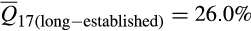 vs.
vs. 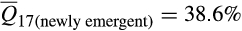 ; t = 20.56; p < .0001). Increases in European wild boar associations were offset by decreases in contributions from Western heritage breeds (
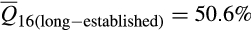 vs.
vs. 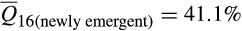 ; t = −16.18; p < .0001) and commercial breeds (
 vs.
vs. 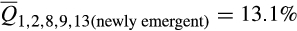 ; t = −8.354; p < .0001).
Concomitant with admixed ancestry, invasive feral swine were genetically diverse with average observed heterozygosity rates across all individuals modestly higher than heterozygosity rates among reference samples ( vs.
vs.  ; p < .0001; Figure 4). Comparisons of observed heterozygosity between long-established and newly emergent populations revealed a modest decrease in genetic diversity among newly emergent populations (
 vs.
vs.  ; p < .0001).

4 DISCUSSION
The recent and rapid expansion of invasive feral swine throughout the contiguous US has been associated with the propagation of individuals of mixed domestic and wild ancestry. Secondary introductions from established invasive populations, as opposed to novel introductions from distinct genetic lineages, have facilitated the expansion of this ecologically and economically destructive IAS over the past 30 years. Specifically, less than 3% (154/6,566) of sampled feral swine could be attributed to the influences of contemporary propagule pressure associated with the release or escape of commercial or heritage domestic breeds, European wild boar, companion animals, or the direct descendants of these distinct lineages. In contrast, invasive feral swine from both long-established and newly emergent populations overwhelmingly were of admixed ancestry with dominant ancestral contributions from Western heritage breeds and European wild boar. Other authors have noted that connectivity among feral swine populations and patterns of range expansion, in particular, reflect human-mediated movement as opposed to natural dispersal, with new populations emerging beyond dispersal distances characterized for the species relative to the previous extent of the invaded range (Bevins et al., 2014; Hernández et al., 2018; Mayer, 2018; McCann et al., 2018; Tabak, Piaggio, Miller, Sweitzer, & Ernest, 2017). Building upon this work, our documentation of the geographical spread of a common, admixed genotype throughout the contiguous US unequivocally demonstrates that secondary introductions from established populations to uninvaded habitats have served as the dominant pathway contributing to recent expansion of the invaded range.
In considering the genetic make-up of feral swine, the results of our ancestry analysis differed substantially from historical accounts of introduction pressure (Mayer & Brisbin, 1991). Mayer and Brisbin (1991) detailed a long and sustained history of domestic pig introductions into the contiguous US. Free-range pig husbandry, a common practice from the time of European colonization to the mid-1900s, served as a potential source for the continuous augmentation of extant populations or establishment of new invasive populations (Mayer, 2018). The genetic make-up of domestic pigs raised under free-range husbandry practices over this period most closely resembled Western heritage breeds organized into reference cluster 16 (Mayer & Brisbin, 1991; White, 2011). In contrast, wild boar introductions have been far more restricted and generally associated with initial importations from native European populations to stock game farms (Mayer & Brisbin, 1991). The disparity in introduction pressure between these two lineages, yet the sizable contribution of European wild boar to the overall genetic composition of modern invasive feral swine ( = 31.7%; significant association for 6,637/6,566 individuals), demonstrates that limited wild boar introductions have had a disproportionate effect on the genetic attributes of invasive feral swine (Mayer & Brisbin, 1991; McCann et al., 2018).
Consistent with the admixed ancestry of invasive feral swine, genetic analyses in other systems are revealing that invasive populations are often of admixed origins (van Boheemen et al., 2017; Kolbe et al., 2004; Lavergne & Molofsky, 2007). Introductions from multiple distinct lineages can offset the genetic decline anticipated among invasive populations due to founder effects and the loss of genetic diversity due to drift during the establishment period. Furthermore, the blending of genetic attributes from disparate lineages enables the emergence of unique phenotypic combinations (Lavergne & Molofsky, 2007). With natural selection acting upon enriched phenotypic diversity, populations can evolve to have heightened invasive ability as a cumulative measure of fitness of invasive populations (Lavergne & Molofsky, 2007). Accordingly, the proliferation of European wild boar ancestry among invasive feral swine populations despite limited initial introductions could be attributable to fitness advantages conveyed by unique behavioural or morphological characteristics of domestic pig–wild boar hybrids. Furthermore, increases in wild boar ancestry among newly emergent feral swine populations could result from the intensification of environmental selective pressures if the fitness advantages of individuals with wild boar phenotypic attributes become greater as limiting factors, such as winter severity, become more restrictive with northward and inland range expansion (McClure et al., 2015; Snow et al., 2017). Support for the assertion that domestic pig–wild boar hybrids may be highly invasive can be drawn from the observed introgression of domestic pigs into native European wild boar populations and subsequent proliferation of admixed genotypes among wild populations in Europe (Fulgione et al., 2016; Goedbloed, Hooft, et al., 2013; Goedbloed, Megens, et al., 2013). Intensive artificial selection imposed during the domestication process has served to dramatically increase the fecundity of domestic pigs relative to wild boar (Miller, 2017). Among wild boar populations in southern Italy, sows of admixed domestic pig–wild boar ancestry have litters that are 40% larger than nonintrogressed wild boar (Fulgione et al., 2016). Such increases in fecundity, despite being accompanied by other morphological traits presumed to be deleterious to survival in the wild (e.g., coat colour or spotted coat pattern), may serve as a mechanism contributing to the heightened invasion potential of feral swine of hybrid ancestry (Fulgione et al., 2016).
Rates of establishment and expansion for invasive feral swine populations that descend from distinct genetic lineages versus populations of admixed ancestry provide further insight into the relative invasion potential for these disparate introduction processes (Estoup & Guillemaud, 2010). Although primary introductions associated with the deliberate or accidental release of domestic pigs, wild boar or companion animals were rare, the detection of such individuals (n = 154; classified based on  ≥ 0.85) in 50 counties across 18 states demonstrates the presence of sustained propagule pressure from these distinct genetic lineages (Appendices S1 and S3). Furthermore, 23 of these introductions occurred in counties where feral swine were not otherwise present and putatively would remain genetically isolated after establishment. Reconciling patterns of population establishment with the ancestry classification of feral swine can elucidate the relative invasion potential of distinct ancestral lineages. Of the 23 counties in which individuals were introduced from distinct lineages, feral swine were eliminated from 21 of those counties over the course of this study (M. Lutman, National Feral Swine Damage Management Program, personal communication). In contrast, the number of counties occupied by feral swine of admixed heritage breed–wild boar ancestry has increased from 768 in 1988 to 2,621 in 2017 (Southeastern Cooperative Wildlife Disease Study, 2015). This rapid expansion of feral swine of admixed ancestry in contrast to the rarity of populations that descend from distinct lineages suggests admixed populations are more successful invaders than those that independently descend from distinct lineages.
Similarly, among long-established invasive feral swine populations, deviations from the pervasive pattern of admixed heritage breed–wild boar ancestry were largely restricted to Mohave County (Arizona) and Florida. Populations in both Mohave County and Florida demonstrated complex ancestries, although patterns of admixture were largely restricted to contributions from reference clusters associated with domestic breeds as opposed to contributions from wild boar (Mohave County, n = 99,  ; Florida, n = 990;
  ). Mayer and Brisbin (1991) attributed the establishment of the Mohave County population to a release of domestic pigs from a nearby ranch before 1900. Patterns of ancestry among Mohave County feral swine corroborate the historical account with consistent associations to Western heritage breeds (cluster 16) and domestic breeds (clusters 1 [Berkshire], 8 [Duroc and related breeds] and 2 [Hampshire]). However, five of the 99 individuals sampled in Mohave County had ancestry associations more typical of feral swine from elsewhere within the invaded range of the contiguous US (i.e., mixed ancestry descending from reference clusters 16 and 17), suggesting recent immigration from another invasive population. By contrast, Florida has a long history of invasive feral swine with populations in the contiguous US first established within the state in the 16th century (Hernández et al., 2018; Zadik, 2000). Mayer and Brisbin (1991) document multiple wild boar or wild boar hybrid introductions into the state, but wild boar ancestry does not appear to have proliferated as elsewhere, with contemporary populations maintaining a strong association to Western heritage breeds (
 ).
).
Although these lines of anecdotal evidence suggest populations of admixed heritage breed–wild boar ancestry have greater invasion potential than populations independently established from distinct genetic lineages, patterns of artificial selection similarly could contribute to the proliferation of wild boar ancestry in the absence of any direct fitness advantages. Specifically, the preferential selection of populations with wild boar phenotypic traits as source populations for secondary introductions—a practice that was common among wildlife management agencies from the 1950s to the 1970s and continues to be common as a result of illegal introductions conducted by private citizens—could amplify wild boar ancestry without genetic influences on invasion potential (Mayer, 2018; Mayer & Brisbin, 1991; McCann et al., 2018; Tabak et al., 2017). Ongoing research to evaluate the influences of ancestry on various measures of fitness and invasion potential (i.e., survival, fecundity, habitat use patterns and dispersal rates) across a range of environmental conditions will help elucidate how processes of natural versus artificial selection are driving the proliferation of genetic associations with European wild boar among North American feral swine populations.
Recently developed genomic tools allowed us to elucidate the complexity of the invasion process contributing to the expansion of one of the most globally destructive IAS (Lowe et al., 2000). Specifically, populations of invasive feral swine of admixed ancestry have expanded rapidly over the past 30 years. In contrast, only a modest number of populations descend directly from primary introductions despite evidence of sustained propagule pressure from distinct genetic lineages (154 invasive feral swine samples attributable to the release of domestic breeds, wild boar or companion animals). Furthermore, feral swine ancestry deviated from historical accounts of domestic pig and wild boar introductions, demonstrating that the limited number of wild boar introductions have had a disproportionate effect on the genetic composition of invasive populations. Finally, the proliferation of feral swine of admixed heritage breed–wild boar ancestry in the US and reciprocal introgression of domestic breeds into European wild boar populations suggests admixed individuals may have heightened invasion potential relative to independent introductions from distinct genetic lineages (Fulgione et al., 2016; Goedbloed, Hooft, et al., 2013; Goedbloed, Megens, et al., 2013). The greater invasion potential of populations with admixed wild and domestic origins, relative to populations that descend from distinct lineages, has important implications for both the evolutionary dynamics and management of this IAS. As invasive feral swine are among the most broadly distributed mammals in the world, similar ancestry analyses in other regions could help inform whether the unique combination of phenotypes produced with the hybridization of domestic and wild lineages represents an essential evolutionary shift for free-range populations of S. scrofa to become invasive (Lewis et al., 2017). Artificial selection exerted over the past 9,000 years has broadened phenotypic variation within S. scrofa beyond that typically found in natural systems. The admixture of domestic and wild lineages within invasive populations, as documented here and elsewhere (Barrios-Garcia & Ballari, 2012), may then expand the functional diversity that is then acted upon by natural selection throughout the invasion process. With a broad array of phenotypic variation represented among domestic and wild lineages, a long history of global introductions, and the capacity to use our understanding of direct linkages between genotypes and phenotypes, feral swine are emerging as a model system to describe the evolution of invasive populations.
ACKNOWLEDGEMENTS
We thank Courtney Pierce, Anna Mangan, Hannah Walker, Blake McCann, Mark Wilburn and Katherine McClure for suggestions on the manuscript. Research was supported by the National Feral Swine Damage Management Program, the National Wildlife Disease Program and the National Wildlife Research Center.
AUTHOR CONTRIBUTIONS
T.J.S. and A.J.P. designed and performed the research, produced and analysed the data, and composed the manuscript. M.A.T., C.S., M.S.R. and R.S.M. designed the research, analysed the data and composed the manuscript. M.B., H.-J.M., M.A.M.G., S.R.P., D.A.dF., H.D.B. and B.S.S. produced the data and composed the manuscript.
Open Research
DATA AVAILABILITY STATEMENT
A complete listing of all reference samples and associated metadata (sample name, reference group, reference cluster and citation for published genotypes) is provided in Appendix S2. A complete list of invasive feral swine samples, associated metadata (state, county and date of collection) and ancestry vectors are provided in Appendices S1, S3 and S6. Genotypes for invasive feral swine and reference samples are available as well as all r scripts developed to execute the described analyses through the Dryad data repository (https://doi.org/10.5061/dryad.jsxksn05z).