Tracking climate change in the spatial distribution pattern and the phylogeographic structure of Hyrcanian wood frog, Rana pseudodalmatina (Anura: Ranidae)
Amiri and Vaissi contributed equally to this work.
Contributing authors: Negar Amiri ([email protected]), Somaye Vaissi ([email protected]), Fateme Aghamir ([email protected]), Reihaneh Saberi-Pirooz ([email protected]), Dennis Rödder ([email protected]), Elham Ebrahimi ([email protected])
Abstract
Climate change has essential effects on patterns of population persistence, connectivity, and divergence. We used mtDNA sequences and species distribution modeling to assess the impact of climatic changes in the past (Last Glacial Maximum [LGM: 21 Kya] and Mid-Holocene [6 Kya]), recent (1970–2000), and future (2070) on the phylogeography and spatial distribution of populations of the Hyrcanian wood frog, Rana pseudodalmatina, in northern Iran. Based on two mitochondrial genes (cytochrome b and 16S ribosomal RNA), we found evidence for two regional patterns that diverged in the Pleistocene (1.6 Mya) and are distributed in the eastern and western sections of the current species range. Biogeographic analyses support the hypothesis that both vicariance (an increase in the Caspian Sea water levels) and dispersal events have been involved in shaping the species' genetic structure. Reconstruction of the ancestral distribution of R. pseudodalmatina suggests the species' range contracted in two independent eastern and western glacial refugia during the LGM, expanding from the Mid-Holocene to the present to occupy Hyrcanian forests continuously. According to future climate projections, the species' range shows a tendency to shift to higher altitudes. Landscape connectivity analyses support higher population continuity in the central part of the current range, with isolated populations in the easternmost and westernmost extremes. Our integrative study of R. pseudodalmatina provides support for the “refugia-within-refugia” scenario in the Hyrcanian forests.
1 INTRODUCTION
Climatic changes through time have important effects on the evolutionary history and spatial distribution of species (Bontrager & Angert, 2019; Foden et al., 2013; Hopley & Byrne, 2019; Omann et al., 2009; Razgour et al., 2019; Velásquez-Tibata et al., 2012; Vieira et al., 2018). Historical changes in regional climate also play an important role in conditioning patterns of gene flow among populations, with species-specific life histories and demographics also contributing to shaping species distributions and their temporal dynamics (Baek et al., 2018; Bell et al., 2010; Hua, 2013; Safner et al., 2011; Schierenbeck, 2017). Numerous phylogeographic studies have shown that during cold phases of the last glacial period the distribution ranges of many species contracted to climatic refugia (Bao et al., 2015; Leipold et al., 2017; Malekoutian et al., 2020; Song et al., 2018). Subsequently, as temperatures increased during the Holocene, distributions expanded again to occupy newly suitable habitats (Chen et al., 2017; Cox et al., 2019; Igea et al., 2013; Liepelt et al., 2009; Zhao et al., 2019). On shorter, more recent time scales, climate change has been linked to distribution shifts in many species, sometimes resulting in local or regional extinction (Devictor et al., 2012; He et al., 2018; McCarty, 2001). According to 131 studies, extinction rates in response to climate change are estimated to range from 0% to 54%, with an average of 7.9% (Urban, 2015). Therefore, understanding how species respond to climate change is of fundamental importance in conservation planning.
Identifying Quaternary climatic refugia due to stable climatic conditions can be critical to the conservation of species for future climate change in terms of predicting the effects on population persistence (Provan & Bennett, 2008), especially in globally threatened groups like amphibians (Alroy, 2015; Duarte et al., 2012; Pounds et al., 2006). Due to their biphasic life-cycles, highly permeable skin, and unshelled eggs, amphibians are particularly vulnerable to alterations in environmental conditions, and climate change has been identified as one of the most important factors threatening their populations (Carey & Alexander, 2003; Corn, 2005; Wake & Vredenburg, 2008). Amphibians are regarded as good bioindicators of environmental changes due to their physiological constraints and relatively low mobility (Carnaval et al., 2009). Genetic studies can provide evidence for historical distribution shifts of amphibian populations in response to climatic oscillations during the Quaternary (Afroosheh et al., 2019; Chiocchio et al., 2017; Fouquet et al., 2012; Provan & Bennett, 2008; Yodthong et al., 2015; Zeisset & Beebee, 2008; Zhang et al., 2016; Zhou et al., 2014). Integrative studies combining phylogeographic analyses with species distribution modeling (SDM) can be used to assess the impact of past climatic changes on the evolutionary history and historical demography of populations and help predict future changes in their geographical ranges (Afroosheh et al., 2019; Ahmadzadeh et al., 2013; Nicolas et al., 2018; Velo-Antón et al., 2013).
The Hyrcanian wood frog, Rana pseudodalmatina Eiselt & Schmidtler, 1971, is a brown frog (Anura, Ranidae) endemic to temperate forests in northern Iran (also known as Hyrcanian forests). It ranges from the Talesh region to the Golestan National Park, on the northern slopes of the Alborz Mountains and the southern edge of the Caspian Sea of Iran (Najibzadeh et al., 2018). The species composition and diversity of the Southwest Asian forests, rich in endemic species, suggests that the Hyrcanian region has likely acted as a glacial refugium for many taxa during the Quaternary glaciations (Röhrig, 1991; Saberi-Pirooz et al., 2018). Phylogeographic studies and climatic models have shown that the southern Caspian Sea has acted as a glacial refugium for a broad range of taxa, including Iranian rock lizards (Darevskia chlorogaster and Darevskia defilippii, Ahmadzadeh, Flecks, et al., 2013), Iranian brown bears (Ursus arctos, Ashrafzadeh et al., 2016), fat dormouse (Glis glis, Ahmadi et al., 2018), Persian mountain salamanders (Paradactylodon persicus, Ahmadzadeh et al., 2020), and Caspian green lizard (Lacerta strigata, Saberi-Pirooz et al., 2021). During the last half-century, the climate became warmer in the Hyrcanian forests, with the average annual temperature increasing between 1.28 and 2.45℃ and annual precipitation declining between 55.6 and 409.4 mm (Tohidifar et al., 2016). Due to the close relationship between temperature and rainfall and amphibian distributions (Ortiz-Yusty et al., 2013), this warming trend is expected to have a negative impact on the distribution of R. pseudodalmatina. This species is categorized as Least Concern (LC) in the IUCN Red List, but few studies have assessed the species’ conservation status and threats (Sharifi et al., 2009).
The main aims of this study are (a) to investigate the evolutionary history and demographic history of R. pseudodalmatina based on two mitochondrial DNA fragments (cytochrome b, cytb, and 16S ribosomal RNA, 16S); (b) to assess the impact of past (Last Glacial Maximum and Mid-Holocene) and more recent (1970–2000) climate fluctuations on the spatial distribution pattern of the species using Species Distribution Models (SDMs); and (c) to investigate whether R. pseudodalmatina will behave as a single distributional unit in response to future climate change (2070).
2 MATERIALS AND METHODS
2.1 Sampling
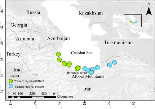
Twenty specimens of R. pseudodalmatina and five specimens of Rana macrocnemis were collected across their distribution range in the Hyrcanian forests (Figure 1, Appendix 1). Tissue samples consisted of third toe clips; all sampled individuals were subsequently released at the site of capture. Samples were preserved in 96% ethanol and kept at −20℃ prior to DNA extraction. Details of sampling locations, accession numbers for newly generated mtDNA sequences, and code ID are presented in Appendix 1.
2.2 Laboratory procedures and sequence analysis
DNA was extracted following a standard high-salt protocol (Sambrook, 1989). The primers L14841 (Kocher et al., 1989)/CB3H and 16SA/16SB (Palumbi et al., 1991) were used to amplify fragments of two mitochondrial genes: Cytochrome b (cytb; 700 bp) and 16S ribosomal RNA (16S; 560 bp), respectively (Table S1). PCRs were run in a total volume of 25 µl containing 12.5 µl of Master Mix Red (Ampliqon), 0.5 µl of each primer (10 µM), 10.5 µl ddH2O, and 1 µl of template DNA. Amplification of each gene was carried out under the conditions described in Veith et al. (2003) (see Table S1). PCR amplifications were visualized on 1% agarose gels including negative controls. PCR products were sequenced by Macrogen Inc. Chromatographs were checked and edited using Codon-Code Aligner v.6.0.2.X (CodonCode Corporation). All new sequences were submitted to GenBank (Appendix 1).
2.3 Phylogenetic analysis
For phylogenetic analysis, some sequences were obtained from the NCBI (www.ncbi.nlm.nih.gov) and were added to our dataset (see Appendix 1). The sequences of the two mtDNA genes (cytb and 16S) were aligned with MAFFT v.6 (Katoh et al., 2017) (https://mafft.cbrc.jp/; algorithm: Auto; scoring matrix: 200 Pam/k = 2; Gap open penalty: 1.53) and were then combined, resulting in a 937 bp alignment (cytb: 442 bp; Alignment S1 and 16S: 495 bp; Alignment S2). The best-fit model was selected using MrModeltest v.2.3 (Nylander, 2004) under Akaike's information criterion (Akaike, 1974). GTR+G+I (Rodriguez et al., 1990; Yang, 1996) was selected as the best-fit model for both cytb and 16S genes (G = 1.05 and p-inv = 0.55; G = 0.47 and p-inv = 0.41). A maximum likelihood (ML) tree was reconstructed using RAxML v.7.2 (Stamatakis, 2006) under the GTR+G+I model with 1000 bootstrap pseudoreplicates to assess branch support. The Bayesian inference (BI) analysis was performed using MrBayes v.3.2 (Huelsenbeck & Ronquist, 2001) with two simultaneous runs and four chains with 107 generations. We subsampled trees and parameters every 100th generation, which produced 105 trees. The first 10% of these trees were discarded as burn-in, and the remaining trees were used to reconstruct a consensus tree. The final standard deviation (SD) of split frequencies for the combine dataset (two genes) was 0.0015. The parameters were separately calculated for each gene partition. We assessed run performance, convergence of parameters, and effective sample size (ESS) with Tracer v.1.6 (Rambaut et al., 2007). The statistical significance of alternative tree topologies using the Shimodaira-Hasegawa (SH) (Shimodaira & Hasegawa, 1999) was evaluated with 1000 bootstrap pseudoreplicates likelihood ratio test (SH-aLRT; Anisimova et al., 2011) as implemented in IQ-Tree v.1.6.12 (Nguyen et al., 2015).
Uncorrected p-distances between two western and eastern groups (see results) were calculated with PAUP v.4.0a10 (Swofford, 2002) for each mtDNA gene separately.
2.4 Estimating divergence time
The divergence times were estimated with BEAST v.1.7.2 (Drummond & Rambaut, 2007) using the combined data set (cytb and 16S). For calibration of the molecular clock, a secondary calibration approach was taken based on two calibration points: first, we set the age for the R. pseudodalmatina/R. macrocnemis – Rana tavasensis clade at 5.18 million years ago (Mya) based on Ehl et al. (2019); and second, we set the time of the most recent common ancestor (henceforth MRCA) of Rana arvalis, Rana temporaria, and Rana pyrenaica at 7.68 Mya, based on Ehl et al. (2019). These calibration points were applied as follows: first node, normal distribution, mean: 5.18 Mya, standard deviation: 1.42 Mya; second node, normal distribution, mean: 7.68 Mya, standard deviation: 1.68 Mya. Analyses were run under a lognormal relaxed clock (uncorrelated) model, because primary runs using an uncorrelated lognormal clock revealed ucld. stdev (δ > 0.1) for all genes. The Yule process was used as a prior for the speciation process. The analysis was run for 3 × 10⁷ generations, sampling trees and parameters every 103 generations. Tracer v.1.5 was used to assess convergence and effective sample sizes (ESS) of parameter estimates.
2.5 Genetic structure and demographic analysis
An analysis of molecular variance (AMOVA) was conducted based on standardized estimates of genetic differentiation (Fst) with 10,000 permutations to assess genetic structure in R. pseudodalmatina using Arlequin v.3.5 (Excoffier & Lischer, 2010). Molecular diversity indices, including the number of haplotypes (H), haplotype diversity (h), and nucleotide diversity (π), were assessed for both markers separately using the same program.
The historical demography of the two regional patterns (see results) in R. pseudodalmatina was investigated with neutrality analyses, calculating Tajima's D and Fu's Fs indices with Arlequin v.3.5. Additionally, mismatch distributions (MMD) were reconstructed using the same software, comparing the frequency distribution of pairwise nucleotide differences in cytb sequences in each regional pattern, with that expected under sudden demographic expansion.
As a complementary approach, we reconstructed the Bayesian skyline plots (BSP; Drummond et al., 2005) to investigate the variations in effective population size (henceforth Ne) through time, in each regional pattern, using cytb sequences. The analysis was conducted with BEAST v1.7.2 under a strict molecular clock model with a fixed rate of 1.8 × 10⁻² substitutions per site per Mya (estimated for the related brown frog R. arvalis, Babik et al., 2004). The analysis was run for 5 × 10⁶ generations with parameters sampled every 100 iterations. The parsimony haplotype network was constructed using TCS v.1.21 (Clement et al., 2000) for the cytb sequences under the 95% limit of parsimony.
2.6 Biogeographic analysis
Based on the results of phylogenetic analyses (see section 3), the distribution of R. pseudodalmatina can be divided into two areas, corresponding to the western (W) and eastern (E) sections of the species range. The statistical dispersal-vicariance analysis (S-DIVA) and Bayesian binary MCMC (BBM) analysis were used to reconstruct the possible ancestral range for R. pseudodalmatina. The analysis was implemented using RASP v.2.1 beta (Yu et al., 2015) using cytb sequences. Because this analysis requires a fully resolved topology, we used a reduced tree including only haplotypes (see Appendix 1) as input for the analysis. The haplotype tree was used as input for the analysis. To consider phylogenetic uncertainty, 20,000 of the posterior trees sampled during the BI analyses were used as the input file for S-DIVA. The BBM analysis was run for 5 × 10⁶ generations under 10 MCMC, and the sampling frequency was every 100 generations. The fixed Jukes-Cantor model with equal among-site rate variation was used for the BBM analysis.
2.7 Potential distribution analysis (past–present–future)
2.7.1 Species record, climate data, and variable selection
We compiled information on georeferenced localities of R. pseudodalmatina from our own fieldwork and literature sources (Appendix 1). When no coordinates were provided in literature sources, we georeferenced the observations using the Biogeomancer Software (http://bg.berkeley.edu/latest/). In total, 41 unique records were available for model building covering the whole known geographic range of the species, which were mapped in ArcGIS v.10.8 to spot potential errors.
Climatic information characterizing current climatic conditions was obtained from WorldClim.org v.2.0 in terms of 19 bioclimatic predictors with a spatial resolution of 2.5 arc.min (Fick & Hijmans, 2017). To reduce the multi-collinearity of predictors, we used the SDMtune package for Cran R (Vignali et al., 2020) to identify a set of variables that have low collinearity and at the same time a high predictive ability for the study species. The final set of variables were as follows: BIO7 = Temperature Annual Range; BIO8 = Mean Temperature of Wettest Quarter; BIO9 = Mean Temperature of Driest Quarter; BIO13 = Precipitation of Wettest Month.
To estimate past and future range dynamics, we followed two different approaches: (a) We used downscaled global circulation model outputs for the time slices Mid-Holocene (6 ky BP) and at the Last Glacial Maximum (LGM; 21 ky BP) as unweighted ensembles based on palaeoclimate simulations following the r1i1p1 ensemble from the PMIP3 project (Paleoclimate Modeling Intercomparison Project Phase III, https://pmip3.lsce.ipsl.fr/; (Braconnot et al., 2012). A total of 11 scenarios were available as estimates of Mid-Holocene climate (MRICGCM3, MPI-ESM-P, MIROC-ESM, IPSL-CM5A-LR, GISS-E2-R, FGOALS-g2, CSIRO-Mk3l-1-2, CSIRO-Mk3-0, CNRM-CM5, CCSM4, and BCC-CSM1-1) and seven scenarios were available for the LGM (MRI-CGCM3, MPI-ESM-P, MIROC-ESM, IPSL-CM5A-LR, FGOALS-g2, CNRM-CM5, and CCSM4). To evaluate the potential future distribution in 2070, we used averages of four IPCC 5 storylines RCP 2.6, RCP 4.5, RCP 6, and RCP 8.5 as suggested by 10 GCMs (NorESM1-M, MRI-CGCM3, MIROC5, MIROC-ESM, MIROC-ESM-CHEM, IPSL-CM5A-LR, HadGEM2-ES, HadGEM2-AO, GISS-E2-R, CCSM4, and BCC-CSM1-1). The downscaling procedure to 2.5 arc.min is described in Krehenwinkel et al. (2016). (b) As the second climate data set we used Oscillayers provided by Gamisch (2019). This dataset comprises 256-time slices in steps of 10 ky characterizing climatic oscillations within the Pleistocene. For each time slice, 19 bioclimatic variables with a spatial resolution of 2.5 arc.min are available which are conceptually equivalent to those available from WorldClim.
2.7.2 Species distribution modeling
For SDM development, we used MaxEnt v.3.4.4 (Phillips et al., 2006, 2017), which is a presence-pseudoabsence method and allows an estimation of potentially suitable habitats (Elith et al., 2011). To identify the most suitable settings, we used the relevant functions of the SDMtune package (Vignali et al., 2020), which suggested a regulation parameter of 0.5 and linear, quadratic, and product features. The total number of species records was 100 times split into 20% used for model testing via the area under the receiver operating characteristic curve (AUC; Swets, 1988) and 80% used for model training applying a bootstrap procedure. Averages across all replicates were projected to current climatic conditions as well as past time slices using the cloglog output format. As environmental background for model training, we selected an area defined by a circular buffer of 75 km enclosing all species records. As a presence–absence threshold, we used an omission threshold of 10% acknowledging potential georeferencing errors. As projecting SDMs through space and time may be subject to extrapolation errors in areas with environmental conditions exceeding the training range of the model, we used multivariate environmental similarity surfaces (MESS; Elith et al., 2010) to quantify areas with increased projection uncertainties. Potential refugia were identified by overlaying all potential distributions as projected onto the oscillayer dataset. Stable refugia were classified as 100% present across all 256-time slices, 99%, 95%, and 90%. Based on this stability through time map, potential gene flow among populations was estimated using Circuitscape v5 (McRae et al., 2008).
3 RESULTS
3.1 Phylogenetic analysis
Based on the combined datasets (cytb and 16S; 937 bp), the BI consensus and ML bootstrap trees showed R. pseudodalmatina as siter group to a clade containing R. macrocnemis, Rana holtzi, and R. tavasensis (Figure S1). Furthermore, the monophyly of R. pseudodalmatina is well supported (BS = 99; SH-aLRT = 100; PP = 1.00), and two regional patterns are recognized within the species distribution range in the east (E) and west (W) (Figure S1, Figure 1).
Based on the cytb and 16S, uncorrected genetic distances between E and W groups were low, 0.8% and 0.3%, respectively.
3.2 Estimating divergence time
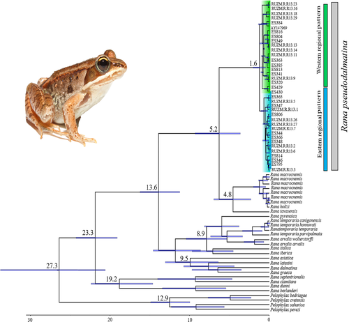
Based on the combined mtDNA genes, the MRCA of Hyrcanian/Anatolia lineage and other species of the genus Rana in Europe lived at 13.6 Mya (95% HPD; 6.23–21.11 Mya). At the intra-species level, R. pseudodalmatina haplotypes shared a MRCA at 1.6 Mya (95% HPD; 0.58–2.54 Mya; Figure 2).
3.3 Genetic structure and demographic analysis
Molecular diversity indices based on the cytb and 16S genes including the number of H, h, and π within R. pseudodalmatina and its regional patterns are presented in Table 1. The cytb fragment contained 16 variable sites (12 transitions and four transversions), of which seven were parsimony-informative and nine were singletons. The mean nucleotide composition was A: 22.91%, T: 27.61%, C: 33.76%, and G: 15.73%. The 16S fragment contained 16 variable sites (14 transitions and two transversions), of which one was parsimony-informative and 15 were singletons. Mean nucleotide composition was A: 29.79%, T: 25.27%, C: 24.33%, and G: 20.61%.
| Gene | N | H | h | π | Tajima's D | Fu's Fs | |
|---|---|---|---|---|---|---|---|
| Rana pseudodalmatina | cytb | 39 | 12 | 0.78 | 0.005 | −0.52 | −2.07 |
| 16S | 48 | 13 | 0.69 | 0.002 | −2.15* | −9.28* | |
| E | cytb | 17 | 4 | 0.50 | 0.0008 | −1.04 | −1.47* |
| 16S | 19 | 6 | 0.46 | 0.001 | −2.04* | −3.86* | |
| W | cytb | 22 | 8 | 0.60 | 0.001 | −2.07* | −4.42* |
| 16S | 29 | 7 | 0.37 | 0.001 | −2.28* | −4.68* |
- * p < 0.05.
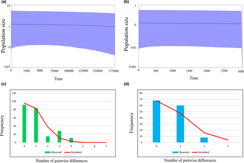
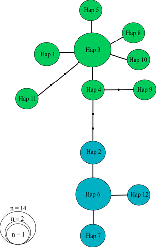
AMOVA results showed significant genetic differences between two regional patterns (E and W) based on mtDNA genes (cytb: Fst = 0.44, p < 0.05; 16S: Fst = 0.58, p < 0.05). Most values of Tajima's D and Fu's Fs in R. pseudodalmatina and its regional patterns were significant and negative (Table 1). The MMD diagrams for the E and W displayed a unimodal pattern with right-skewed consistent with recent demographic expansion (Figure 3c, d). The BSP based on cytb showed no obvious trends in Ne through time in each regional pattern (Figure 3a, b). The haplotype parsimony network for the cytb gene showed that the western and eastern groups were separated from each other with two-step mutations (Figure 4).
3.4 Biogeographic analysis
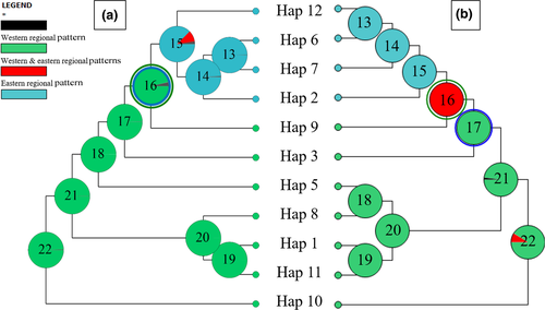
Ancestral distributions of R. pseudodalmatina were inferred from S-DIVA and BBM analyses (Figure 5). In both reconstructions, the most recent common ancestor of the species was distributed in the Hyrcanian forests; subsequently, it expanded into the western and eastern areas. According to S-DIVA, a vicariance event took place in the ancestral node of the two areas, and dispersal occurred in the western distribution. BBM reconstruction indicated that vicariance and dispersal events shaped the species’ current distribution (Figure 5).
3.5 Species distribution modeling (past–present–future)
The potential distributions as suggested by our models for past (Last Glacial Maximum, LGM [21 Kya] and Mid-Holocene [6 Kya]), current (1970–2000), and future (2070) climatic conditions are shown in Figure 6, and Figure S2, wherein the average performance was AUCtest = 0.828. On average, Temperature Annual Range (BIO7: 57.3%) had the highest contribution, followed by Precipitation of Wettest Month (BIO13: 25.2%), Mean Temperature of Wettest Quarter (BIO8: 9.0%), and Mean Temperature of Driest Quarter (BIO9: 8.5%).
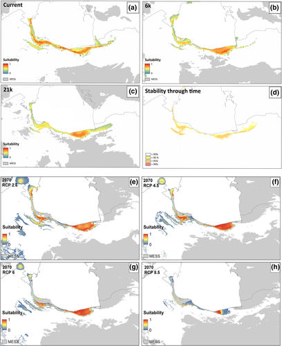
Based on the SDMs, the central part of the Caspian coast in the southern region was identified as most suitable habitats for R. pseudodalmatina during the LGM (Figure 6c). But in the Mid-Holocene, the potential distribution range of the species expanded to include the eastern, central, and western Hyrcanian forests (Figure 6c). Under current climatic conditions, the potential range of the species increased, with habitat suitability uniformly expanding in the Hyrcanian forests from the Talesh region to the Golestan National Park on the southern edge of the Caspian Sea and in the northern slopes of the Alborz Mountains (Figure 6a).
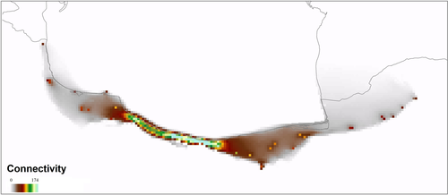
According to the RCPs 2.6, 4.5, 6, and 8.5 scenarios of future climate projections, the distribution range of R. pseudodalmatina would tend to shift to higher altitudes especially in the western part of the range in the northern slope of Alborz Mountain (Figure 6e-h). Stability through time suggests that the Hyrcanian forests acted as historical refugia for this species (Figure 6d). Based on landscape analyses, connectivity under current climatic conditions is maximum in the central part of the range and decreases in the easternmost and westernmost extremes (Figure 7).
4 DISCUSSION
We examined the genetic diversity patterns of the Hyrcanian wood frog, R. pseudodalmatina, throughout its geographic range in the Hyrcanian forests. Also, we used phylogeography and species distribution modeling approaches to investigate the putative glacial refugia and the effect of climate oscillations on the species.
We analyzed two mtDNA genes (cytb and 16S) and found the Hyrcanian/Anatolian lineage and other species of the genus Rana in Europe had MRCA during the Miocene (13.6 Mya: 95% HPD; 6.23–21.11 Mya; Figure 2). It is assumed that the uplift of the Turkish–Iranian plateau and the physical vicariance such as the salt-water barrier may have led to the speciation among the Anatolian, the Caucasian, and the Iranian brown frogs (Najibzadeh et al., 2017). Rana pseudodalmatina displayed a phylogeographic pattern with two regional groups across its distribution range in the western and eastern Hyrcanian forests (Figure 1, Figure S1). The results of Najibzadeh et al. (2018) corroborate our findings that the species forms two distinct groups in the east and west of the geographic range. However, Najibzadeh et al. (2017) estimate of TMRCA of the two groups is older compared to our findings. Nevertheless, the authors noted that their methodology is prone to misleading results. According to our result, the MRCA of two regional patterns lived 1.6 Mya (95% HPD; 0.58–2.54 Mya), which is much more recent compared to the equivalent estimate of Najibzadeh et al. (2020), which was ca. 4 Mya. This difference is possibly due to the different set of markers, the number of individual samples, prior settings, and calibration points used in the two studies. We used two mtDNA markers (cytb and 16S) for divergence time estimations; however, Najibzadeh et al. (2020) only used the 16S gene. Our estimated divergence time is comparable to the Caspian green lizard (L. strigata) and Fat Dormouse (Gilis gilis) that turned into the eastern and western lineages about 0.9 Mya (95% HPD: 0.55–1.16 Mya) and 1.19 Mya (95% HDP: 0.55–1.91 Mya), respectively, in the Hyrcanian region (Ahmadi et al., 2018; Saberi-Pirooz et al., 2021).
According to the AMOVA results, the two populations are almost isolated from each other because of the Fst value of nearly 0.5. The MRCA of the two regional groups of R. pseudodalmatina was during the Pleistocene (1.6 Mya [95% HPD; 0.58–2.54 Mya]; Figure 2), which suggests that this species may have been affected by the Quaternary climate fluctuations. It seems that the presence of two groups of R. pseudodalmatina in the west and east of the distribution may indicate the long-term residence within two different glacial refugia during the Pleistocene. The existence of cryptic refugia and the idea of “refugia-within-refugia” in the Hyrcanian forests that is proposed here for R. pseudodalmatina has been previously discussed for other species that live in this region (Ahmadi et al., 2018; Ahmadzadeh, Flecks, et al., 2013; Saberi-Pirooz et al., 2021). The assessments of demographic history revealed that the recent expansion occurred in the populations (Table 1 and Figure 3).
Our findings identified a successive vicariance event correspond to the divergence of the regional eastern and western groups from the ancestral node (Figure 5). We suggested that the increase in the Caspian Sea water level during the Pleistocene led to the occurrence of vicariance event for the species (Lateef, 1998; Mamedov, 1997). On the other hand, the results of S-DIVA and the BBM analysis showed that dispersal events also played an important role in creating this disjunct distribution pattern (Figure 5). The parsimony haplotype network based on the cytb gene indicated that the more derived haplotypes were found in the western region (Figure 4). This suggested that the species derived from the west of the Hyrcanian forests and then migrated to the east of the distribution area.
In response to climate change, species shifted their distribution range to reach more favorable conditions (Guedes et al., 2020). Based on SDMs results, R. pseudodalmatina showed a scenario of past range contraction followed by recent expansion (Figure 6 and Figure S2). We assumed during the LGM, the distribution of the R. pseudodalmatina has been concentrated in two different glacial refugia in the east and west of the distribution range (Figure 6c). Given the warmer conditions since the Mid-Holocene compared to the recent climatic conditions (Akhani et al., 2010), its distribution in the more suitable habitat and a longitudinal shift was expanded throughout the Hyrcanian forests (Figure 6a,b). The longitudinal shift of the distribution range is also shown in the study of Duan et al. (2016) on Chinese amphibians.
The optimal temperatures for R. pseudodalmatina range between 11 and 18℃, and species activity decreases widely at temperatures above 23℃ (Pesarakloo et al., 2012). According to our result, Temperature Annual Range (BIO7) had the highest contribution in the model in the past, recent, and future climate change (57.3%). Based on the future climate (2070) projection, the distribution range of the R. pseudodalmatina will shift upward to higher altitudes in the northern slope of Alborz Mountains where the species currently occurs (Figure 6). The results of our study confirm the general trend that amphibian species migrate to higher altitudes under the influence of climate warming. For example, Forero-Medinaet al. (2011) investigated 46 amphibian species of tropical mountains and showed that under future climate changes, their range of distribution will shift to higher altitudes. In contrast to these trends and our findings, Najibzadeh et al. (2020) showed that the suitable habitat for R. pseudodalmatina has remained stable since the LGM and will remain the same in the future.
Based on the results of the Circuitscape analysis, the highest connectivity was observed between the populations located in the central parts (the westernmost part of the eastern regional population) to the westward (the easternmost part of the western regional population) of Mazandaran (Figure 7). These results may indicate secondary (postglacial) contact of these populations (Austin et al., 2004; Zamudio & Savage, 2003), which requires further investigation in future studies. According to the results of the stability map through time in this study, Hyrcanian forests acted as climate refugia for the R. pseudodalmatina during climate change (Figure 6d). Therefore, Hyrcanian forests may be buffered to contemporary climate change over time and provide resistance to valued socio-cultural, ecological, and physical resources.
ACKNOWLEDGEMENTS
We would like to thank HG Kami for providing some samples. We would also like to thank Saeedeh Ataei, Mahshid Oladi, and Yasaman Ranjbaran for their help in improving the manuscript. We thank too Paschalia Kapli for accommodating comments on an earlier adaptation of the original copy.
CONFLICT OF INTEREST
There are no conflicts of interest.
APPENDIX 1
The dataset of Rana used in this study. The information includes code ID, haplotype number for cytb (HT cytb), locality, origin, geographical coordinates and the accession numbers for two mtDNA (cytb and 16S) genes
| Taxon | HT cytb | Locality/Country | Lat (N)/Long (E) | Origin | GenBank accession numbers | |
|---|---|---|---|---|---|---|
| code ID | 16S | cytb | ||||
| Rana pseudodalmatina | ||||||
| ES365 | — | Iran/Golestan | 37.035/55.03 | This study | MT864022 | — |
| ES347 | Hap 2 | Iran/Golestan | 36.9944/55.0599 | This study | MT864026 | MW017119 |
| ES349 | — | Iran/Mazandaran | 36.533/51.532 | This study | MT864010 | — |
| ES363 | Hap 3 | Iran/Mazandaran | 36.225/51.366 | This study | MT864012 | MW017121 |
| ES320 | Hap 4 | Iran/Mazandaran | 36.662/51.184 | This study | MT864028 | MW017117 |
| ES341 | — | Iran/Mazandaran | 36.369/51.133 | This study | MT864009 | — |
| ES344 | Hap 6 | Iran/Mazandaran | 36.458/52.997 | This study | MT864019 | MW017118 |
| ES346 | — | Iran/Mazandaran | 36.365/52.36 | This study | MT864020 | — |
| ES348 | Hap 6 | Iran/Mazandaran | 36.68/53.53 | This study | MT864021 | MW017120 |
| ES366 | Hap 6 | Iran/Mazandaran | 36.57/52.032 | This study | MT864023 | MW017122 |
| ES795 | Hap 2 | Iran/Mazandaran | 36.082/52.823 | This study | MT864015 | MW017125 |
| ES804 | — | Iran/Mazandaran | 36.523/51.091 | This study | MT864016 | — |
| ES806 | Hap 7 | Iran/Mazandaran | 36.089/36.089 | This study | MT864024 | MW017126 |
| ES814 | — | Iran/Mazandaran | 36.654/53.598 | This study | MT864025 | — |
| ES813 | — | Iran/Mazandaran | 36.67/51.188 | This study | MT864017 | — |
| — | Hap 3 | Iran/Mazandaran | — | Veith et al. (2003) | — | AY147969 |
| ES384 | Hap 1 | Iran/Gilan | 36.992/50.081 | This study | MT864011 | MW017123 |
| ES385 | — | Iran/Gilan | 36.992/50.081 | This study | MT864013 | — |
| ES816 | Hap 3 | Iran/Gilan | 37.137/49.665 | This study | MT864018 | MW017127 |
| ES429 | Hap 5 | Iran/Gilan | 37.66/48.92 | This study | MT864014 | MW017124 |
| ES430 | — | Iran/Gilan | 37.67/48.91 | This study | MT864027 | — |
| RUZM.R.R13.1 | Hap 6 | Iran/Loveh | 37.35/55.65 | Najibzadeh et al. (2018) | MF344713 | MF344774 |
| RUZM.R.R13.2 | Hap 6 | Iran/Loveh | 37.35/55.65 | Najibzadeh et al. (2018) | MF344714 | MF344775 |
| RUZM.R.R13.3 | Hap 6 | Iran/Loveh | 37.35/55.65 | Najibzadeh et al. (2018) | MF344715 | MF344776 |
| RUZM.R.R13.4 | Hap 6 | Iran/Loveh | 37.35/55.65 | Najibzadeh et al. (2018) | MF344712 | MF344773 |
| RUZM.R.R13.5 | Hap 6 | Iran/Behshahr | 36.66/53.59 | Najibzadeh et al. (2018) | MF344716 | MF344777 |
| RUZM.R.R13.6 | Hap 6 | Iran/Behshahr | 36.66/53.59 | Najibzadeh et al. (2018) | MF344717 | MF344778 |
| RUZM.R.R13.7 | Hap 6 | Iran/Behshahr | 36.66/53.59 | Najibzadeh et al. (2018) | MF344718 | MF344779 |
| RUZM.R.R13.8 | Hap 6 | Iran/Behshahr | 36.66/53.59 | Najibzadeh et al. (2018) | MF344719 | MF344780 |
| RUZM.R.R13.9 | Hap 8 | Iran/Rasht | 37.15/49.52 | Najibzadeh et al. (2018) | MF344720 | MF344781 |
| RUZM.R.R13.11 | Hap 3 | Iran/Rasht | 37.15/49.52 | Najibzadeh et al. (2018) | MF344721 | MF344782 |
| RUZM.R.R13.12 | Hap 3 | Iran/Rasht | 37.15/49.52 | Najibzadeh et al. (2018) | MF344722 | MF344783 |
| RUZM.R.R13.13 | Hap 3 | Iran/Rasht | 37.15/49.52 | Najibzadeh et al. (2018) | MF344723 | MF344784 |
| RUZM.R.R13.14 | Hap 9 | Iran/Rasht | 37.15/49.52 | Najibzadeh et al. (2018) | MF344724 | MF344785 |
| RUZM.R.R13.15 | Hap 3 | Iran/Rasht | 37.15/49.52 | Najibzadeh et al. (2018) | MF344725 | MF344786 |
| RUZM.R.R13.16 | Hap 3 | Iran/Salmanshahr | 36.64/51.19 | Najibzadeh et al. (2018) | MF344726 | MF344787 |
| RUZM.R.R13.17 | Hap 3 | Iran/Salmanshahr | 36.64/51.19 | Najibzadeh et al. (2018) | MF344727 | MF344788 |
| RUZM.R.R13.18 | Hap 10 | Iran/Astara | 38.34/48.83 | Najibzadeh et al. (2018) | MF344728 | MF344789 |
| RUZM.R.R13.19 | Hap 3 | Iran/Astara | 38.34/48.83 | Najibzadeh et al. (2018) | MF344729 | MF344790 |
| RUZM.R.R13.21 | Hap 3 | Iran/Astara | 38.34/48.83 | Najibzadeh et al. (2018) | MF344730 | MF344791 |
| RUZM.R.R13.22 | Hap 3 | Iran/Astara | 38.34/48.83 | Najibzadeh et al. (2018) | MF344731 | MF344792 |
| RUZM.R.R13.23 | Hap 11 | Iran/Astara | 38.34/48.83 | Najibzadeh et al. (2018) | MF344732 | MF344793 |
| RUZM.R.R13.24 | Hap 3 | Iran/Astara | 38.34/48.83 | Najibzadeh et al. (2018) | MF344733 | MF344794 |
| RUZM.R.R13.25 | Hap 6 | Iran/Sari | 36.33/52.60 | Najibzadeh et al. (2018) | MF344735 | MF344796 |
| RUZM.R.R13.26 | Hap 7 | Iran/Sari | 36.33/52.60 | Najibzadeh et al. (2018) | MF344736 | MF344797 |
| RUZM.R.R13.27 | Hap 12 | Iran/Sari | 36.33/52.60 | Najibzadeh et al. (2018) | MF344734 | MF344795 |
| RUZM.R.R13.28 | Hap 3 | Iran/Langarud | 37.17/50.16 | Najibzadeh et al. (2018) | MF344737 | MF344798 |
| RUZM.R.R13.29 | Hap 1 | Iran/Langarud | 37.17/50.16 | Najibzadeh et al. (2018) | MF344738 | MF344799 |
| Rana macrocnemis | ||||||
| ES405 | Iran/Azerbijan | This study | MZ171537 | MW017128 | ||
| ES407 | Iran/Azerbijan | This study | — | MW017129 | ||
| ES416 | Iran/Azerbijan | This study | MZ171538 | MW017130 | ||
| ES419 | Iran/Azerbijan | This study | MZ171539 | MW017131 | ||
| ES420 | Iran/Azerbijan | This study | MZ171540 | MW017132 | ||
| Veith et al. (2003) | AY147940 | AY147960 | ||||
| Rana arvalis arvalis | Veith et al. (2003) | AY147938 | AY147958 | |||
| Rana arvalis wolterstorffi | Veith et al. (2003) | AY147939 | AY147959 | |||
| Rana macrocnemis | Veith et al. (2003) | AY147940 | AF373151 | |||
| Rana dalmatina | Veith et al. (2003) | AY147944 | AY147962 | |||
| Rana graeca | Veith et al. (2003) | AY147945 | — | |||
| Rana holtzi | Veith et al. (2003) | AY147946 | AY147964 | |||
| Rana iberica | Veith et al. (2003) | AY147947 | AY147965 | |||
| Rana pyrenaica | Peso-Fernández et al. (2016) | KU720300 | KU720300 | |||
| Rana temporaria temporaria | Veith et al. (2003) | AY147956 | AY147977 | |||
| Rana temporaria parvipalmata | Veith et al. (2003) | AY147955 | AY147976 | |||
| Rana temporaria canigonensis | Veith et al. (2003) | AY147952 | AY147973 | |||
| Rana temporaria honnorati | Veith et al. (2003) | AY147954 | AY147975 | |||
| Rana italica | Veith et al. (2003) | AY147948 | — | |||
| Rana italica | Canestrelli et al. (2008) | — | EU595505 | |||
| Rana latastei | Veith et al. (2003) | AY147949 | AY147967 | |||
| Rana asiatica | Yuan et al. (2016) | KX269200 | KX269346 | |||
| Rana dalmatina | Canestrelli et al. (2014) | — | KJ789718 | |||
| Rana italica | Canestrelli et al. (2008) | — | EU595490 | |||
| Rana tavasensis | Veith et al. (2003) | — | AY147970 | |||
| Rana berlandieri | Hillis and Wilcox (2005)/Yuan et al. (2016) | AY779235 | KX269301 | |||
| Rana dunni | Hillis and Wilcox (2005)/Yuan et al. (2016) | AY779222 | KX269305 | |||
| Rana clamitans | Hillis and Wilcox (2005)/Yuan et al. (2016) | AY779204 | KX269304 | |||
| Rana septentrionalis | Yuan et al. (2016) | KX269179 | KX269314 | |||
| Pelophylax bedriagae | Hofman et al. (2016) | NC-029200 | NC-029200 | |||
| Pelophylax perezi | Vences (1999)/Busack and Lawson (2008) | AF215424 | DQ902145 | |||
| Pelophylax saharica | Lymberakis et al. (2007) | DQ474229 | DQ902147 | |||
| Pelophylax cretensis | Hofman et al. (2016) | NC-025575 | NC-025575 | |||


