Volume 44, Issue 4 pp. 418-436

Original Article

Open Access

Geometric ergodicity and conditional self-weighted M-estimator of a GRCAR( $p$ ) model with heavy-tailed errors

Xiaoyan Li,

Xiaoyan Li

College of Mathematics and Statistics, Chongqing University, Chongqing, 401331 China

Search for more papers by this author

Jiazhu Pan,

Corresponding Author

Jiazhu Pan

[email protected]

orcid.org/0000-0001-7346-2052

Department of Mathematics and Statistics, University of Strathclyde, Glasgow, G1 1XH UK

Correspondence to: Jiazhu Pan, Department of Mathematics and Statistics, University of Strathclyde, 26 Richmond Street, Glasgow G1 1XH, UK.

Email: [email protected]

Search for more papers by this author

Anchao Song,

Anchao Song

School of Public Health and Management, Chongqing Medical University, Chongqing, 400016 China

Search for more papers by this author

Xiaoyan Li,

Xiaoyan Li

College of Mathematics and Statistics, Chongqing University, Chongqing, 401331 China

Search for more papers by this author

Jiazhu Pan,

Corresponding Author

Jiazhu Pan

[email protected]

orcid.org/0000-0001-7346-2052

Department of Mathematics and Statistics, University of Strathclyde, Glasgow, G1 1XH UK

Correspondence to: Jiazhu Pan, Department of Mathematics and Statistics, University of Strathclyde, 26 Richmond Street, Glasgow G1 1XH, UK.

Email: [email protected]

Search for more papers by this author

Anchao Song,

Anchao Song

School of Public Health and Management, Chongqing Medical University, Chongqing, 400016 China

Search for more papers by this author

First published: 19 January 2023

https://doi.org/10.1111/jtsa.12680

Share a link

Email
Wechat
Bluesky

Abstract

We establish the geometric ergodicity for general stochastic functional autoregressive (linear and nonlinear) models with heavy-tailed errors. The stationarity conditions for a generalized random coefficient autoregressive model (GRCAR( $p$ )) are presented as a corollary. And then, a conditional self-weighted M-estimator for parameters in the GRCAR( $p$ ) is proposed. The asymptotic normality of this estimator is discussed by allowing infinite variance innovations. Simulation experiments are carried out to assess the finite-sample performance of the proposed methodology and theory, and a real heavy-tailed data example is given as illustration.

1 INTRODUCTION

Suppose that

\{y_{t}, t \geq 1 - p\}

are observations from the generalized random coefficient autoregressive (GRCAR) model with order

p

defined by

y_{t} = ϕ_{t 0} + ϕ_{t 1} y_{t - 1} + ϕ_{t 2} y_{t - 2} + \dots + ϕ_{t p} y_{t - p} + ε_{t}, t = 1, 2, \dots

(1)

where

{{(ϕ_{t}^{'}, ε_{t})}^{'} = {(ϕ_{t 0}, ϕ_{t 1}, \dots, ϕ_{t p}, ε_{t})}^{'}, t \geq 1}

is a sequence of independent and identically distributed (i.i.d.) random vectors with

E ϕ_{t} = ϕ = {(ϕ_{0}, ϕ_{1}, \dots, ϕ_{p})}^{'}

. Here, it is assumed that

{(ϕ_{t}^{'}, ε_{t})}^{'}

is independent of

ℱ_{t - 1} = σ (y_{t - 1}, y_{t - 2}, \dots, y_{1 - p})

. We are interested in stationarity of the above model and estimation of unknown parameter vector

ϕ = {(ϕ_{0}, ϕ_{1}, \dots, ϕ_{p})}^{'}

with its true value

ϕ_{0}

. Note that, in model (1), the random coefficients are permitted to be correlated with the error process.

Model (1) with $p = 1$ (GRCAR(1)) was first introduced by Hwang and Basawa (1998), and it includes Markovian bilinear model and random coefficient exponential autoregressive model as special cases. When $V a r (ϕ_{t}) = 0$ , model (1) becomes the ordinary autoregressive (AR( $p$ )) model. There have been a lot of perfect theoretical achievements about it. For example, Ling (2005) proposed a self-weighted least absolute deviation estimator and showed its asymptotic normality. The method has been used in many references, such as Pan et al. (2007), Pan and Chen (2013), Pan et al. (2015). Wang and Hu (2017) proposed a self-weighted M-estimator for the AR(p) model and established the asymptotic normality of this estimator. When $V a r (ϕ_{t}) \neq 0$ with $p = 1$ , and $ϕ_{t}$ is independent of $ε_{t}$ , model (1) becomes the first-order random coefficient autoregressive (RCAR(1)) model (see Nicholls and Quinn (1982)), which has been frequently used to describe the random perturbations of dynamical systems in economics and biology (see Tong (1990), Yu et al. (2011), Zhang et al. (2015), Araveeporn (2017)). As a generalization of RCAR model and AR models, GRCAR model has become one type of important models in nonlinear time series, since it allows dependence between random errors and random coefficients. Estimation of parameters and asymptotic properties of GRCAR models have been studied in the literature. For instance, Hwang and Basawa (1997) established the local asymptotic normality of a class of GRCAR models. Zhao and Wang (2012) constructed confidence regions for the parameters by using empirical likelihood method. Zhao et al. (2013) considered the problem of testing the constancy of coefficients in a GRCAR model by empirical likelihood method. Zhao et al. (2018) studied the variable selection problem in GRCAR models. Zhao et al. (2019) proposed a weighted least squares estimate and empirical likelihood (EL) based weights through using some auxiliary information for GRCAR models. Moreover, time series models with heavy-tailed errors, even when $E ({ε_{t}}^{2})$ is infinite, are often found and studied in economic and financial modeling. Wu (2013) studied M-estimation for general ARMA processes with infinite variance. Yang and Ling (2017) investigated the self-weighted least absolute deviation estimation for heavy-tailed threshold autoregressive models. Fu et al. (2021) studied the asymptotic properties for the conditional self-weighted M-estimator of GRCAR(1) model with possibly heavy-tailed errors. However, general easy-to-check conditions for stationarity and limiting distributions of robust parameter estimators for statistical inference of GRCAR( $p$ ) with heavy-tailed errors are still open problems.

This article aims to reach two targets. First, we establish the geometric ergodicity of general stochastic functional autoregressive (linear and nonlinear) models with possibly heavy-tailed error terms under a mild moment condition. Moreover, the stationarity conditions for GRCAR( $p$ ) are implied as a corollary of our general result. Second, motivated by Yang and Ling (2017), Ling (2005), Wang and Hu (2017) and Fu et al. (2021), we prove the asymptotic property of a self-weighted M-estimator (SM-estimator) for GRCAR( $p$ ) with possible infinite variance, and show that the limiting distribution of SM-estimator is asymptotically normal. Simulation results and a real data example are given to support our methodology.

The contents of this article are organized as follows. Section 2 presents the main results. Section 3 reports the simulation results. Section 4 shows a real data example. All proofs of our main results are given in Section 5.

2 MAIN RESULTS

2.1 Geometric Ergodicity

We first establish geometric ergodicity of general stochastic functional autoregressive models (including linear and nonlinear) under a mild moment condition. Then the geometric ergodicity which can imply the stationarity conditions of model (1) is given as a corollary of the main theorem.

Consider a general stochastic functional autoregressive model defined as follows

\{\begin{matrix} y_{t} = φ_{t} (y_{t - 1}, \dots, y_{t - p}) + ε_{t}, t \geq 1 \\ {(y_{0}, y_{- 1}, \dots, y_{- p + 1})}^{'} \in ℛ^{p}, \end{matrix}

(2)

where

{φ_{t}}

is a sequence of i.i.d. stochastic functions such that

\{{(φ_{t} (\cdot), ε_{t})}^{'}\}

being of i.i.d. random vectors, and

{(φ_{t} (\cdot), ε_{t})}^{'}

is independent of

ℱ_{t - 1} = σ (y_{t - 1}, y_{t - 2}, \dots, y_{1 - p})

. It can be seen that both linear and nonlinear autoregressive models are included. This model can be rewritten in vector form as follows:

\{\begin{matrix} X_{t} = Φ_{t} (X_{t - 1}) + ε_{t} U, t \geq 1, \\ X_{0} \in ℛ^{p}, \end{matrix}

(3)

where

Φ_{t} (X_{t - 1}) = {(φ_{t} (y_{t - 1}, \dots, y_{t - p}), y_{t - 1}, \dots, y_{t - p + 1})}^{'}, X_{t} = {(y_{t}, \dots, y_{t - p + 1})}^{'}, U = {(1, 0, \dots, 0)}^{'}

Under the above conditions, model (3) is a homogeneous Markov chain. It is easily seen that stationarity for

\{y_{t}, t \geq 1 - p\}

is equivalent to that for

\{X_{t}, t \geq 0\}

. Furthermore, the geometric ergodicity for model (2) is equivalent to that for the model (3).

Theorem 2.1.Suppose model (3) satisfies

(i)
There exists some norm ${‖\cdot‖}_{v}$ on the p-dimensional vector space,constants $0 < ρ < 1, 0 < δ < 1$ and $c \geq 0$ , such that
$E {‖Φ_{t} (x)‖}_{v}^{δ} \leq ρ {‖x‖}_{v}^{δ} + c, \forall x \in ℛ^{p};$ (4)
(ii)
The density function of $ε_{t}$ is continuous and positive everywhere,and $E {|ε_{t}|}^{δ} < \infty$ for $δ$ in (i).

Then, model (3) is geometrically ergodic, which implies ${y_{t}}$ in model (2) is stationary and geometrically ergodic.

Under the conditions of Theorem 2.1, more concretely, we have the following corollary.

Corollary 2.2.Suppose model (2) satisfies

(i)
There exists a constant vector $φ = {(φ_{1}, \dots, φ_{p})}^{'}$ and a $0 < δ < 1$ satisfying
$1 - φ_{1} z - \dots - φ_{p} z^{p} \neq 0, |z| \leq 1$ (5)
such that
$\lim_{‖x‖ \to \infty} \frac{E {|φ_{t} (x) - φ^{'} x|}^{δ}}{‖x‖} = 0$ (6)
and for any $K > 0$ ,
$\sup_{‖x‖ \leq K} E {|φ_{t} (x) - φ^{'} x|}^{δ} < \infty .$ (7)
(ii)
The density function of $ε_{t}$ is continuous and positive everywhere,and $E {|ε_{t}|}^{δ} < \infty$ for $δ$ in (i).

Then, ${y_{t}}$ in model (2) is stationary and geometrically ergodic.

In Corollary 2.2, when $φ_{t} (x) = ϕ_{t 0} + {(ϕ_{t 1}, \dots, ϕ_{t p})}^{'} x, x \in ℛ^{p}$ , we can get the stationarity conditions for GRCAR( $p$ ) as another corollary of our general result.

Corollary 2.3.Suppose model (1) satisfies

(C.1)
- (i)
  $1 - ϕ_{1} z - \dots - ϕ_{p} z^{p} \neq 0$ , for $|z| \leq 1$ ;
- (ii)
  $E {|ϕ_{t i} - ϕ_{i}|}^{δ} < \infty, i = 1, 2, \dots, p, E {|ϕ_{t 0}|}^{δ} < \infty$ , for a constant $0 < δ < 1$ ;
- (iii)
  The density function of $ε_{t}$ is continuous and positive everywhere, and $E {|ε_{t}|}^{δ} < \infty$ for $δ$ in (ii).
  
  Then, ${y_{t}}$ in model (1) is stationary and geometrically ergodic.

Remark 1.Theorem 2.1 establishes the geometric ergodicity of general stochastic functional autoregressive (linear and nonlinear) models with possibly heavy-tailed error terms under a mild moment condition. The stationarity conditions for GRCAR( $p$ ) in Corollary 2.3 is a consequence of Theorem 2.1. In Corollary 2.3, the moment condition is very weak. We only require a finite moment of order $δ (0 < δ < 1)$ about the error $ε_{t}$ , which includes the Cauchy distribution. The condition on random coefficients makes the model not too far away from the linear AR. This is a reasonable requirement for any (non-parametric or parametric) AR-type model.

Remark 2.We note that the GRCAR is a quite broad kind of models for time series data. A special case of this type of models can be used to describe conditionally heteroscedastic structure. For example, consider the model defined as: $y_{t} = (ϕ_{0} + β_{0} ε_{t}) + (ϕ_{1} + β_{1} ε_{t}) y_{t - 1} + ε_{t}$ , $ε_{t} \sim N (0, σ^{2})$ . The conditional mean and conditional variance of this model are

\begin{align} E (y_{t} | ℱ_{t - 1}) = ϕ_{0} + ϕ_{1} y_{t - 1}; \\ V a r (y_{t} | ℱ_{t - 1}) = σ^{2} {(1 + β_{0} + β_{1} y_{t - 1})}^{2} . \end{align}

It is shown that this very special case of the GRCAR has similar function to AR(1)–ARCH(1), but we don't need to restrict the parameters

β_{0}

and

β_{1}

to be non-negative. Furthermore, if the assumption on the distribution of error is changed to

ε_{t} \sim t_{2}

, the model becomes a model with infinite variance.

2.2 Conditional Self-weighted M-estimation

Denote

X_{t - 1} = {(1, y_{t - 1}, \dots, y_{t - p})}^{'}

. Then the model (1) becomes

y_{t} = ϕ_{t}^{'} X_{t - 1} + ε_{t}

, where

ϕ_{t} = {(ϕ_{t 0}, ϕ_{t 1}, \dots, ϕ_{t p})}^{'}

. Define the objective function

L_{n} (ϕ) = \sum_{t = 1}^{n} ω_{t} ρ (y_{t} - ϕ^{'} X_{t - 1}),

(8)

where

ϕ = E (ϕ_{t}) = {(ϕ_{0}, ϕ_{1}, \dots, ϕ_{p})}^{'}

and

ω_{t}

is a positive function which is measurable to

ℱ_{t - 1} = σ (y_{t - 1}, y_{t - 2}, \dots)

and

ρ (\cdot)

is assumed to be a suitable nonnegative convex function. The conditional self-weighted M-estimator

{\hat{ϕ}}_{S M}

ϕ

is defined by

{\hat{ϕ}}_{S M} = \arg \min_{ϕ \in Θ} L_{n} (ϕ)

where

Θ \subset ℛ^{p + 1}

is the parameter space containing the true value

ϕ_{0}

2.3 Asymptotic Normality of SM-estimation

To derive the asymptotic property of

{\hat{ϕ}}_{S M}

, we need the following assumptions:

(C.2)
Let $ρ (\cdot)$ be a convex function on $ℝ$ with left derivative $ψ_{-}$ and right derivative $ψ_{+}$ . Choose a function $ψ$ such that $ψ_{-} \leq ψ \leq ψ_{+}$ .
(C.3)
Suppose that $G (t) : = E ψ (ε_{1} + t)$ exists, $G (t)$ has a derivative $λ > 0$ at $t = 0$ and $G (0) = 0$ .
(C.4)
$E ψ^{2} (ε_{1}) = τ < \infty$ and $E {(ψ (ε_{1} + t) - ψ (ε_{1}))}^{2} \to 0$ , as $t \to 0$ .
(C.5)
$ω_{t} = g (y_{t - 1}, \dots, y_{t - p})$ is a measurable and positive function on $ℝ^{p}$ such that $E (ω_{t} + {ω_{t}}^{2}) (‖ X_{t} ‖ + {‖ X_{t} ‖}^{2}) < \infty$ , where $‖ v ‖$ denotes the Euclidean norm of a vector $v$ .

Theorem 2.4.Under the (C.1)–(C.5),we have

\sqrt{n} ({\hat{ϕ}}_{S M} - ϕ_{0}) \overset{L}{\to} N (0, \frac{τ}{λ^{2}} \sum^{- 1} Ω \sum^{- 1})

(9)

where

\sum = E (ω_{t} X_{t} {X_{t}}^{'})

Ω = E ({ω_{t}}^{2} X_{t} {X_{t}}^{'})

and

\overset{L}{\to}

denotes convergence in distribution.

Remark 3.Assumption (C.1) does not rule out the possibility that $ε_{t}$ has an infinite variance, and even $E | ε_{t} |$ is infinite. Theorem 2.4 establishes the asymptotic property of SM-estimators for parameters in GRAR( $p$ ) models with possible heavy-tailed errors.

Remark 4.It is worth mentioning that Assumptions (C.2)–(C.4) are traditional assumptions for an M-estimation in a linear model, which can be found in many references, for examples, Bai et al. (1992), Wu (2007) and Wang and Zhu (2018). Examples of $ρ (x)$ satisfying assumptions include $ρ (x) = x^{2}, ρ (x) = |x|$ and $ρ (x) = \frac{1}{2} x^{2} I (|x| \leq m) + (m |x| - \frac{1}{2} m^{2}) I (|x| > m)$ , which then correspond to the conditional self-weighted least-squares estimator, conditional self-weighted least absolute deviation estimator and conditional self-weighted Huber estimator respectively. Assumption (C.5) is standard on the weight $ω_{t}$ for the self-weighted method in IVAR models which allows $E {y_{t}}^{2}$ to be infinite by properly choosing weight function $ω_{t}$ . Firstly, the purpose of the weight $ω_{t}$ is to downweight the leverage points in $X_{t}$ such that the covariance matrices $Ω$ and $\sum$ in Theorem 2.4 above are finite. Secondly, the $ω_{t}$ allow us to approximate $L_{n} ({\hat{ϕ}}_{n})$ by a quadratic form. In addition, Theorem 2.4 generalizes the results of Ling (2005), Wang and Hu (2017) and Fu et al. (2021).

Remark 5.For the case $ρ (x) = x^{2}$ and $E {ε_{1}}^{2} = σ^{2} < \infty$ , taking $ψ (x) = 2 x, λ = 2$ . Applying Theorem 2.4, we have

\sqrt{n} ({\hat{ϕ}}_{S M} - ϕ_{0}) \overset{L}{\to} N (0, σ^{2} \sum^{- 1} Ω \sum^{- 1})

(10)

which shows the asymptotic property of the conditional self-weighted least-squares estimator of parameters in a GRCAR(

p

) model with finite variance.

For the case

ρ (x) = | x |

and

E {ε_{1}}^{2} = \infty

, taking

ψ (x) = s i g n (x)

. Suppose that the errors

ε_{t}

have zero median with a density

f (x)

satisfying

\sup_{x \in R} | f^{'} (x) | < \infty

. Then

λ = 2 f (0)

and

τ = 1

. Using Theorem 2.4, we have

\sqrt{n} ({\hat{ϕ}}_{S M} - ϕ_{0}) \overset{L}{\to} N (0, \frac{1}{4 f {(0)}^{2}} \sum^{- 1} Ω \sum^{- 1})

(11)

which shows the asymptotic property of the conditional self-weighted least absolute deviation estimator for a GRCAR(

p

) model with infinite variance.

For the case

ρ (x) = \frac{1}{2} x^{2} I (|x| \leq m) + (m |x| - \frac{1}{2} m^{2}) I (|x| > m)

, taking

ψ (x) = - m I (x < - m) + x I (|x| \leq m) + m I (x > m)

, and

λ = \int_{- m}^{m} d F (x), τ = m^{2} - \int_{- m}^{m} (m^{2} - x^{2}) d F (x) .

(12)

Using Theorem 2.4, we have

\sqrt{n} ({\hat{ϕ}}_{S M} - ϕ_{0}) \overset{L}{\to} N (0, \frac{τ}{λ^{2}} \sum^{- 1} Ω \sum^{- 1})

(13)

which includes the asymptotic property of the conditional self-weighted Huber estimator for a GRCAR(

p

) model with finite variance or infinite variance.

3 SIMULATION STUDIES

We conduct some simulation studies in finite samples through Monte Carlo experiments. What we are interested in are the accuracy and sampling distribution of the proposed estimator. The results show that our method performs well.

Data are generated from the following GRCAR ( $p$ ) models:

Model A: $y_{t} = (ϕ_{0} + 0.1 ε_{t}) + (ϕ_{1} + 0.1 ε_{t}) y_{t - 1} + ε_{t}$ . Consider $ε_{t} \sim N (0, 1)$ and $ε_{t} \sim t_{2}$ .

Model B: $y_{t} = (ϕ_{0} + 0.1 u_{t}) + (ϕ_{1} + 0.1 u_{t}) y_{t - 1} + ε_{t}$ , where $u_{t} \sim N (0, 1)$ . Consider $ε_{t} \sim N (0, 1)$ , $ε_{t} \sim t_{2}$ and $ε_{t} \sim C a u c h y (0, 1)$ .

The true values of parameters in model A are $(ϕ_{0}, ϕ_{1}) = (0, 0.5)$ , and $(ϕ_{0}, ϕ_{1}) = (0, - 0.5)$ in model B. In model A, the random coefficients are correlated with the error process. The random coefficients are independent of the error process in model B. Here three distributions are given for reference: $N (0, 1)$ has finite expectation and finite variance; $t_{2}$ has finite expectation but infinite variance; Cauchy(0,1) only have a finite moment of order $δ (0 < δ < 1)$ . We set the sample sizes $n = 200$ and $n = 400$ . The number of replications is 2000.

Tables I and II list the biases, standard deviations (SD) and asymptotic standard deviations (ADs) of the conditional self-weighted least absolute deviation estimator (

S M_{1}

) and conditional self-weighted Huber estimator (

S M_{2}

) with the following choice of weight functions respectively:

\begin{align} w_{1 t} = \{\begin{matrix} 1, \begin{matrix}  \end{matrix} | y_{t - 1} | \leq K, \\ \frac{K^{3}}{{|y_{t - 1}|}^{3}}, | y_{t - 1} | > K, \end{matrix} \\ w_{2 t} = I {| y_{t - 1} | \leq K}, \\ w_{3 t} = \frac{1}{1 + {y^{2}}_{t - 1}}, \\ w_{4 t} = \frac{1}{{(1 + y_{t - 1})}^{2}} \end{align}

where

K

is the 0.9 quantile of data

\{| y_{1} |, \dots, | y_{n} |\}

. The weight

w_{1 t}

is similar to Ling (2005). The weights

w_{2 t}, w_{3 t}

and

w_{4 t}

were considered by Yang and Ling (2017). The tuning parameter of Huber estimator is taken as

m = 1.5

. We define

\begin{align} \sum^{^} = \frac{1}{n} \sum_{t = 1}^{n} ω_{t} X_{t} X_{t}^{'}, \hat{Ω} = \frac{1}{n} \sum_{t = 1}^{n} {ω_{t}}^{2} X_{t} X_{t}^{'}, \\ \hat{τ} = \frac{1}{n} \sum_{t = 1}^{n} ψ^{2} ({\hat{ε}}_{t}), \hat{G} (r) = \frac{1}{n} \sum_{t = 1}^{n} ψ ({\hat{ε}}_{t} + r), \end{align}

(14)

\hat{λ}

is the derivative of

\hat{G} (r)

r = 0

and

\{{\hat{ε}}_{t}\}

is the sequence of residuals in GRCAR(

p

). The ADs are calculated by (10)-(14). We estimate

f (0)

{\hat{f}}_{n} (0) = \frac{1}{{\hat{σ}}_{ω} b_{n} n} \sum_{t = 1}^{n} ω_{t} K (\frac{y_{t} - {\hat{ϕ}}_{n}^{'} X_{t - 1}}{b_{n}})

where

{\hat{σ}}_{ω} = \frac{1}{n} \sum_{t = 1}^{n} ω_{t}, K (x) = e^{- x} / {(1 + e^{- x})}^{2}

and

b_{n} = 1.06 \times n^{- 1 / 5}

. For the choice of the optimal bandwidth and its motivation, we refer to Silverman (1986, p. 40) and Pan et al. (2007). Tables I and II show that all the biases are very small and all the SDs and ADs are very close no matter

E {ε_{t}}^{2}

is finite or infinite and no matter the random coefficients are correlated with the error process or independent of the error process. All the biases, SDs and ADs become smaller, when

n

increases from 200 to 400. And the

S M_{2}

estimators perform better than the

S M_{1}

estimators. All of the estimators based on

w_{1 t}

are more efficient than the others.

Table I. Bias, SDs and ADs of the

S M

estimators for model A

			$ε_{t} \sim N (0, 1)$				$ε_{t} \sim t_{2}$
			${\hat{ϕ}}_{0}^{S M_{1}}$	${\hat{ϕ}}_{0}^{S M_{2}}$	${\hat{ϕ}}_{1}^{S M_{1}}$	${\hat{ϕ}}_{1}^{S M_{2}}$	${\hat{ϕ}}_{0}^{S M_{1}}$	${\hat{ϕ}}_{0}^{S M_{2}}$	${\hat{ϕ}}_{1}^{S M_{1}}$	${\hat{ϕ}}_{1}^{S M_{2}}$
$w_{t 1}$	$n = 200$	Bias	0.000	0.000	$- 0.006$	$- 0.005$	0.001	0.001	$-$ 0.004	$-$ 0.005
		SD	0.103	0.084	0.093	0.077	0.123	0.118	0.066	0.065
		AD	0.116	0.075	0.103	0.067	0.137	0.077	0.076	0.043
	$n = 400$	Bias	0.001	0.001	$-$ 0.003	$-$ 0.002	0.001	0.000	$-$ 0.002	$-$ 0.003
		SD	0.072	0.059	0.065	0.053	0.086	0.082	0.044	0.043
		AD	0.079	0.053	0.070	0.047	0.093	0.054	0.051	0.030
$w_{t 2}$	$n = 200$	Bias	0.001	0.001	$-$ 0.002	0.000	0.000	0.002	$-$ 0.008	$-$ 0.007
		SD	0.111	0.090	0.090	0.111	0.132	0.125	0.105	0.099
		AD	0.125	0.081	0.151	0.098	0.114	0.082	0.076	0.064
	$n = 400$	Bias	0.002	0.002	0.001	0.001	0.002	0.002	$-$ 0.003	$-$ 0.002
		SD	0.078	0.064	0.064	0.076	0.092	0.086	0.044	0.065
		AD	0.086	0.057	0.101	0.068	0.076	0.057	0.051	0.044
$w_{t 3}$	$n = 200$	Bias	$-$ 0.001	$-$ 0.001	$-$ 0.003	$-$ 0.004	0.000	0.001	$-$ 0.004	$-$ 0.005
		SD	0.110	0.089	0.095	0.078	0.141	0.134	0.078	0.075
		AD	0.126	0.081	0.107	0.069	0.162	0.090	0.090	0.050
	$n = 400$	Bias	0.000	0.001	$-$ 0.002	$-$ 0.002	$-$ 0.001	0.000	$-$ 0.002	$-$ 0.002
		SD	0.078	0.064	0.067	0.055	0.099	0.093	0.053	0.052
		AD	0.086	0.057	0.073	0.049	0.110	0.063	0.061	0.035
$w_{t 4}$	$n = 200$	Bias	$-$ 0.002	$-$ 0.001	$-$ 0.004	$-$ 0.004	$-$ 0.001	0.002	$-$ 0.004	$-$ 0.005
		SD	0.118	0.096	0.094	0.078	0.152	0.144	0.072	0.070
		AD	0.135	0.087	0.106	0.069	0.174	0.096	0.082	0.046
	$n = 400$	Bias	0.000	0.001	$-$ 0.002	$-$ 0.002	$-$ 0.001	0.000	$-$ 0.002	$-$ 0.002
		SD	0.083	0.068	0.066	0.054	0.106	0.100	0.048	0.048
		AD	0.093	0.061	0.073	0.048	0.119	0.068	0.056	0.032

Table II. Bias, SDs and ADs of the

S M

estimators for model B

			$ε_{t} \sim N (0, 1)$				$ε_{t} \sim t_{2}$				$ε_{t} \sim C a u c h y (0, 1)$
			${\hat{ϕ}}_{0}^{S M_{1}}$	${\hat{ϕ}}_{0}^{S M_{2}}$	${\hat{ϕ}}_{1}^{S M_{1}}$	${\hat{ϕ}}_{1}^{S M_{2}}$	${\hat{ϕ}}_{0}^{S M_{1}}$	${\hat{ϕ}}_{0}^{S M_{2}}$	${\hat{ϕ}}_{1}^{S M_{1}}$	${\hat{ϕ}}_{1}^{S M_{2}}$	${\hat{ϕ}}_{0}^{S M_{1}}$	${\hat{ϕ}}_{0}^{S M_{2}}$	${\hat{ϕ}}_{1}^{S M_{1}}$	${\hat{ϕ}}_{1}^{S M_{2}}$
$w_{t 1}$	$n = 200$	Bias	0.001	$-$ 0.001	0.006	0.006	0.001	0.000	0.005	0.004	0.000	0.000	0.003	0.003
		SD	0.095	0.075	0.092	0.076	0.110	0.106	0.068	0.064	0.127	0.133	0.045	0.044
		AD	0.109	0.075	0.106	0.073	0.131	0.076	0.079	0.046	0.156	0.077	0.045	0.022
	$n = 400$	Bias	0.000	0.001	0.003	0.003	0.000	0.001	0.002	0.002	$-$ 0.002	$-$ 0.002	0.002	0.002
		SD	0.066	0.053	0.065	0.053	0.078	0.075	0.048	0.045	0.090	0.095	0.031	0.031
		AD	0.074	0.053	0.072	0.051	0.089	0.054	0.054	0.032	0.106	0.055	0.031	0.015
$w_{t 2}$	$n = 200$	Bias	0.002	0.000	0.006	0.006	$-$ 0.002	0.000	0.005	0.004	$-$ 0.001	$-$ 0.001	0.005	0.005
		SD	0.102	0.081	0.136	0.110	0.117	0.112	0.097	0.093	0.133	0.138	0.064	0.064
		AD	0.118	0.081	0.155	0.107	0.139	0.081	0.117	0.069	0.161	0.081	0.070	0.035
	$n = 400$	Bias	$-$ 0.001	0.001	0.005	0.004	0.000	0.001	0.003	0.003	$-$ 0.002	$-$ 0.002	0.003	0.003
		SD	0.071	0.058	0.095	0.076	0.083	0.079	0.070	0.067	0.093	0.100	0.044	0.045
		AD	0.080	0.057	0.105	0.074	0.094	0.057	0.080	0.048	0.110	0.057	0.048	0.024
$w_{t 3}$	$n = 200$	Bias	0.000	$-$ 0.001	0.006	0.005	$-$ 0.002	$-$ 0.001	0.004	0.002	0.000	0.000	0.004	0.005
		SD	0.101	0.079	0.094	0.077	0.125	0.121	0.079	0.073	0.164	0.175	0.076	0.073
		AD	0.116	0.079	0.107	0.074	0.150	0.087	0.089	0.052	0.200	0.102	0.072	0.036
	$n = 400$	Bias	$-$ 0.001	0.001	0.002	0.002	$-$ 0.003	$-$ 0.001	0.001	0.001	0.000	0.000	0.002	0.002
		SD	0.070	0.057	0.065	0.053	0.090	0.086	0.055	0.051	0.115	0.124	0.051	0.050
		AD	0.079	0.056	0.073	0.052	0.102	0.062	0.061	0.037	0.136	0.072	0.049	0.026
$w_{t 4}$	$n = 200$	Bias	0.000	$-$ 0.001	0.006	0.005	$-$ 0.003	$-$ 0.001	0.003	0.002	0.001	0.001	0.004	0.005
		SD	0.108	0.085	0.094	0.077	0.136	0.131	0.074	0.068	0.176	0.188	0.066	0.062
		AD	0.125	0.085	0.107	0.074	0.161	0.094	0.082	0.048	0.215	0.109	0.060	0.030
	$n = 400$	Bias	$-$ 0.001	0.001	0.002	0.002	$-$ 0.004	$-$ 0.002	0.001	0.001	0.001	0.001	0.002	0.002
		SD	0.075	0.061	0.065	0.053	0.097	0.092	0.051	0.048	0.125	0.134	0.044	0.043
		AD	0.085	0.060	0.073	0.052	0.110	0.067	0.056	0.034	0.146	0.077	0.041	0.021

To get an overall view on the sampling distributions of the $S M_{1}$ estimators and the $S M_{2}$ estimators, we simulate 2000 replications for the case $ϕ_{1} = 0.5$ and $n = 400$ when the error distributions are $N (0, 1)$ and $t_{2}$ for model A, and for the case $ϕ_{1} = - 0.5$ and $n = 400$ when the error distributions are $N (0, 1)$ , $t_{2}$ and Cauchy for model B. Denote $N_{n 1} = \sqrt{n} ({\hat{ϕ}}_{1}^{S M_{1}} - 0.5) / {\hat{σ}}_{S M_{1}}, N_{n 2} = \sqrt{n} ({\hat{ϕ}}_{1}^{S M_{2}} - 0.5) / {\hat{σ}}_{S M_{2}}$ ; $N_{t 1} = \sqrt{n} ({\hat{ϕ}}_{1}^{S M_{1}} - 0.5) / {\hat{σ}}_{S M_{1}}, N_{t 2} = \sqrt{n} ({\hat{ϕ}}_{1}^{S M_{2}} - 0.5) / {\hat{σ}}_{S M_{2}}; N_{c 1} = \sqrt{n} ({\hat{ϕ}}_{1}^{S M_{1}} - 0.5) / {\hat{σ}}_{S M_{1}}, N_{c 2} = \sqrt{n} ({\hat{ϕ}}_{1}^{S M_{2}} - 0.5) / {\hat{σ}}_{S M_{2}}$ , when the error distribution is $N (0, 1)$ , $t_{2}$ and $C a u c h y$ respectively, where ${\hat{σ}}_{S M_{1}}$ and ${\hat{σ}}_{S M_{2}}$ are the SDs of ${\hat{ϕ}}_{1}^{S M_{1}}$ and ${\hat{ϕ}}_{1}^{S M_{2}}$ respectively. Figure 1 shows the density curves of model A. The density curves of model B are presented in Figure 2. We can see that the density of $N (0, 1)$ is approximated reasonably well by those of $N_{n 1}, N_{n 2}$ , $N_{t 1}, N_{t 2}$ and $N_{c 1}, N_{c 2}$ in both model A and model B.

Details are in the caption following the image — **Figure 1**
Open in figure viewer PowerPoint

The sampling distribution for model A

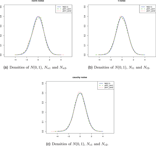
In conclusion, the numeric results show that the conditional self-weighted M-estimators perform well in finite sample no matter with finite variance or infinite variance.

4 REAL DATA ANALYSIS

The proposed methodology is applied to modeling a real dataset. We consider the Hang Seng Index (HSI) for the stock market which is the most influential index in the Hong Kong stock market and one of the most important indices in the Asian financial markets as well. This index has been extensively investigated in the literature. Our dataset consists of the daily Hang Seng closing index from 7 May 2020 to 31 December 2021, which was downloaded at https://cn.investing.com/. There are 412 available observations in total, which are denoted by

x_{1}, x_{2}, \dots, x_{412}

. The first 392 data are selected as the training sample to build model, and next 20 data are used as test sample to evaluate the model. We take the following steps to analyze this dataset by the GRCAR model and method proposed in this article.

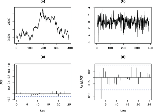
Step 1. Data transformation: The sample time plot for the data ${x_{t}}$ is shown in Figure 3(a). It can be seen that the time series is not stationary because of various levels. To get a stationary time series, let $y_{t} = 100 \times (\log (x_{t} / x_{t - 1}))$ . The sample path plot for the data ${y_{t}}$ is shown in Figure 3(b). Figure 3(b) indicates that ${y_{t}}$ is close to stationarity.
Step 2. Model identification: The plot of sample autocorrelation function (ACF) and sample partial autocorrelation function (PACF) of ${y_{t}}$ are presented in Figure 3(c) and (d) respectively. Figure 3 can provide some important information for tentative identification of the orders of a stable AR model. Based on the sample ACF and PACF plots, it is reasonable to consider fitting an AR(3) autocorrelation structure to ${y_{t}}$ . Since stock data are affected by various factors, the coefficients of the autoregressive model may also change randomly over time, even the coefficients may be correlated with the error, so we can try to fit a GRCAR(3) model instead of AR(3). However, we realize that the data may be heavy-tailed and how to determine the order of autoregression for a time series with infinite variance is a problem which needs further study. Here we just use the sample PACF to give a rough indication of the order in which a GRCAR model might be fitted.
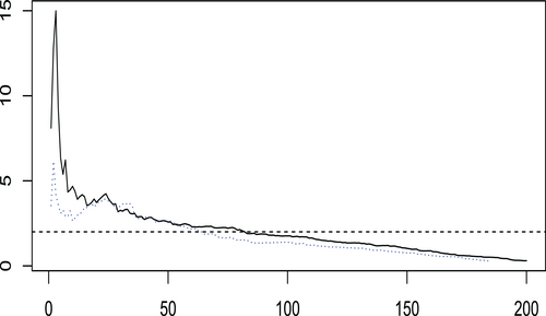
Step 3. Heavy-tail test: To test whether ${y_{t}}$ has a heavy-tailed distribution, we use Hill's estimator (see Drees et al. (2000) and Resnick (2000)) to estimate the tail index of $y_{t}$ . Let $y_{(1)} > y_{(2)} > \dots > y_{(n)}$ be the order statistics of $y_{t}, t = 1, \dots, n$ . The estimators of the right-tail and left-tail indices are defined as
$\begin{align} H_{1 k} = {\{\frac{1}{k} \sum_{i = 1}^{k} \log (\frac{y_{(i)}}{y_{(k + 1)}})\}}^{- 1}, \\ H_{2 k} = {\{\frac{1}{k} \sum_{i = 1}^{k} \log (\frac{y_{(n - i + 1)}}{y_{(n - k)}})\}}^{- 1}, \end{align}$
respectively. Figure 4 displays the Hill estimates of the right-tail and left-tail indices when $1 \leq k \leq 200$ . From Figure 4, we can see that both the right and left tail indices are most likely less than 2. Hence, $y_{t}$ should have a heavy tail. Therefore, it may be more appropriate to suppose these data are generated from a process with infinite variance rather than to assume this data have finite variance.

Based on the above discussion, we can fit a GRCAR(3) model to the data:
$y_{t} = (ϕ_{0} + ε_{t}) + (ϕ_{1} + ε_{t}) y_{t - 1} + (ϕ_{2} + ε_{t}) y_{t - 2} + (ϕ_{3} + ε_{t}) y_{t - 3} + ε_{t}, ε_{t} \sim t_{2} .$ (15)
Step 4. Parameter estimation: The unknown parameters are estimated by different methods on the training data. We calculated the mean absolute errors (MAEs) of predicted values for transformed data based on 1000 repetitions. The results are shown in Table III. From them, we can see that the self-weighted estimators perform better, especially $S M_{2}$ . So we choose the $S M_{2}$ for further analysis. The estimates are
$(ϕ_{0}, ϕ_{1}, ϕ_{2}, ϕ_{3}) = (0.0493, 0.0059, 0.0214, - 0.1608),$
whose corresponding asymptotic standard deviations are $0.0028, 0.0019, 0.0018, 0.0018$ respectively.
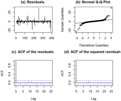
Step 5. Model diagnostics: The absolute value of the eigenvalues for the corresponding matrix in model (15) are 0.5549, 0.5383 and 0.5383, which are all less than one. Therefore, this model satisfies the stationary conditions of Corollary 2.3. Figure 5 presents the residuals of the fitted model (15), the normal $Q$ – $Q$ plot of the residuals, the sample autocorrelation function (ACF) of the residuals and the sample ACF of the squared residuals. From that, we can see the model (15) fits the data reasonably well.
Step 6. Prediction: We use the above model (15) to predict $y_{393}, y_{394}, \dots, y_{412}$ in the test set. As the coefficient of model (15) is random, the predicted values of Hang Seng Index from 3 December 2021 to 31 December 2021, $x_{393}, x_{394}, \dots, x_{412}$ , were calculated by taking the average of 1000 repetitions. We compare our GRCAR(3) model with the AR(3) model and AR(3)-ARCH(2) model. The predictive performance of different models is presented in Figure 6. We can see that the predicted value of model (15) captures the change trend of the real value and most of the predicted values are very close to the true values. Figure 6 and Table IV also show that the GRCAR(3) model performs better than AR(3) model and AR(3)–ARCH(2) model for this dataset.

Table III. Mean absolute errors (MAE) of predicted values on the training set for transformed data

Methods	$S M_{1}$	$S M_{2}$	LAD	LS
MAE	0.9691	0.9529	0.9800	0.9996

Table IV. Some indicators of predictive accuracy on test set about the original data

	Mean of residual	SD of residual	MAE
AR(3)	$- 32.60$	282.93	200.98
GRCAR(3)	8.07	279.34	176.75

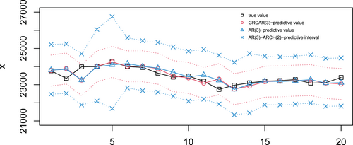
In summary, our model and method perform well in analysis and forecasting of time series data with heavy-tailed distributions.

5 PROOFS OF THEORETICAL RESULTS

This section presents the proofs of our theoretical results.

Proof of Theorem 2.1.It is easy to see that ${X_{t}}$ defined by (3) is a homogenous Markov chain. By the conditions of Theorem 2.1, this Markov chain is $u_{p}$ -irreducible and aperiodic, and all bounded sets with positive $u_{p}$ -measure in $R^{p}$ are small sets. Take the test function $g (x) = {‖x‖}_{v}^{δ}$ . It holds that

\begin{align} E \{g (X_{t})| X_{t - 1} = x\} & = E \{g (Φ_{t} (x) + ε_{t} U)\} \\ = E {‖Φ_{t} (x) + ε_{t} U‖}_{v}^{δ} \\ \leq E {‖Φ_{t} (x)‖}_{v}^{δ} + E {‖ε_{t} U‖}_{v}^{δ} \\ \leq ρ {‖x‖}_{v}^{δ} + c + (E {|ε_{t}|}^{δ}) {‖U‖}_{v}^{δ} \\ = ρ {‖x‖}_{v}^{δ} + c + c^{'} \\ = α {‖x‖}_{v}^{δ} - [(α - ρ) {‖x‖}_{v}^{δ} - c - c^{'}], \end{align}

where

0 < ρ < α < 1, c^{'} = (E {|ε_{t}|}^{δ}) {‖U‖}_{v}^{δ}

. Let

C = \{x : {‖x‖}_{v}^{δ} \leq k\}, k > \max \{1, \frac{c + c^{'}}{α - ρ}\}

, then

C

is a small set, and

\begin{align} E \{g (X_{t})| X_{t - 1} = x\} \leq α {‖x‖}_{v}^{δ} - c_{1}, \forall x \notin C, \\ E \{g (X_{t})| X_{t - 1} = x\} \leq c_{2}, \forall x \in C, \end{align}

where

c_{1} = (α - ρ) k - c - c^{'}, c_{2} = ρ k + c + c^{'}

. By the Lyapunov shift criteria (see Meyn and Tweedie (1994)), the model (3) is geometrically ergodic,which implies

{y_{t}}

in model (2) is stationary and geometrically ergodic.

Proof of Corollary 2.2.We only need to verify the condition (i) of Theorem 2.1. Denote

A = (\begin{matrix} φ_{1} & φ_{2} & \dots & φ_{p - 1} & φ_{p} \\ 1 & 0 & \dots & 0 & 0 \\ 0 & 1 & \dots & 0 & 0 \\ ⋮ & ⋮ & ⋮ & ⋮ & ⋮ \\ 0 & 0 & \dots & 1 & 0 \end{matrix}) .

The condition (5) of Corollary 2.2 is equivalent to

λ^{p} - φ_{1} λ^{p - 1} - \dots - φ_{p} \neq 0, | λ | \geq 1

. It implies the roots

λ_{1}, \dots, λ_{p}

| λ I - A | = 0

satisfy

| λ_{i} | < 1, i = 1, 2, \dots, p

. Put

ρ = \max {| λ_{i} |, i = 1, 2, \dots, p}

, then

0 < ρ < 1

. Thus there exists a positively definite matrix

V_{p \times p}

and

0 < ρ < 1

such that

A^{'} V A \leq ρ^{2} V

(see Ciarlet (1982)). Furthermore,

\forall x \in R^{p}, x^{'} A^{'} V A x \leq ρ^{2} x^{'} V x .

Define a norm

{‖\cdot‖}_{v}

as follows

{‖x‖}_{v} = {(x^{'} V x)}^{1 / 2}, \forall x \in R^{p} .

Then

{‖A x‖}_{v} \leq ρ {‖x‖}_{v}, \forall x \in R^{p} .

Let

H_{t} (x) = Φ_{t} (x) - A x = {(φ_{t} (x) - φ^{'} x, 0, \dots, 0)}^{'}

, where

φ^{'} = (φ_{1}, \dots, φ_{p})

. By the norm equivalence, there is a positive constant

M

such that

\frac{E {‖H_{t} (x)‖}_{v}^{δ}}{{‖x‖}_{v}^{δ}} \leq \frac{M E {‖H_{t} (x)‖}^{δ}}{{‖x‖}^{δ}} = \frac{M E {|φ_{t} (x) - φ^{'} x|}^{δ}}{{‖x‖}^{δ}} .

(16)

By (6), when

‖x‖ \to \infty

, the right-hand side of the above inequality tends to 0. Hence, there exists a constant

K_{0}

such that

E {‖H_{t} (x)‖}_{v}^{δ} \leq \frac{1}{2} (1 - ρ^{δ}) {‖x‖}_{v}^{δ}

for

{‖x‖}_{v}^{δ} > K_{0}

. Therefore,

\begin{align} E ‖ Φ_{t} (x) ‖_{v}^{δ} & = E ‖ A x + H_{t} (x) ‖_{v}^{δ} \\ \leq {‖A x‖}_{v}^{δ} + E {‖H_{t} (x)‖}_{v}^{δ} \\ \leq ρ^{δ} {‖x‖}_{v}^{δ} + E {‖H_{t} (x)‖}_{v}^{δ} \\ \leq \{\begin{array}{l} \frac{1}{2} (1 + ρ^{δ}) {‖x‖}_{v}^{δ}, {‖x‖}_{v}^{δ} \geq K_{0}, \\ ρ^{δ} {‖x‖}_{v}^{δ} + M_{1}, {‖x‖}_{v}^{δ} < K_{0} . \end{array} \end{align}

By (7) and (16), when

{‖x‖}_{v}^{δ} < K_{0}

, there exists a constant

M_{1} \geq 0

such that

E {‖H_{t} (x)‖}_{v}^{δ} \leq M_{1}

. This implies that the condition (i) of Theorem 2.1 holds. By Theorem 2.1, we get the result of this corollary.

Proof of Corollary 2.3.We only need to verify the condition (i) of corollary 2.2.

Define

φ_{t} (x) = ϕ_{t 0} + (ϕ_{t 1}, \dots, ϕ_{t p}) x, x \in R^{p} .

Then

\begin{align} {|φ_{t} (x) - φ^{'} x|}^{δ} & = {|ϕ_{t 0} + (ϕ_{t 1} - ϕ_{1}, \dots, ϕ_{t p} - ϕ_{p}) x|}^{δ} \\ \leq {|ϕ_{t 0}|}^{δ} + {|(ϕ_{t 1} - ϕ_{1}, \dots, ϕ_{t p} - ϕ_{p}) x|}^{δ} . \end{align}

Therefore

\begin{align} \lim_{‖x‖ \to \infty} \frac{E {|φ_{t} (x) - φ^{'} x|}^{δ}}{‖x‖} & \leq \lim_{‖x‖ \to \infty} \frac{E {|ϕ_{t 0}|}^{δ}}{‖x‖} + \lim_{‖x‖ \to \infty} \frac{E {|(ϕ_{t 1} - ϕ_{1}, \dots, ϕ_{t p} - ϕ_{p}) x|}^{δ}}{‖x‖} \\ \leq \lim_{‖x‖ \to \infty} \frac{E {|ϕ_{t 0}|}^{δ}}{‖x‖} + \lim_{‖x‖ \to \infty} \frac{E {‖{(ϕ_{t 1} - ϕ_{1}, \dots, ϕ_{t p} - ϕ_{p})}^{'}‖}^{δ} {‖x‖}^{δ}}{‖x‖} \\ \leq \lim_{‖x‖ \to \infty} \frac{E {|ϕ_{t 0}|}^{δ}}{‖x‖} + \lim_{‖x‖ \to \infty} \frac{E (\sum_{i = 1}^{p} {|ϕ_{t i} - ϕ_{i}|}^{δ}) {‖x‖}^{δ}}{‖x‖} \\ \leq \lim_{‖x‖ \to \infty} \frac{E {|ϕ_{t 0}|}^{δ}}{‖x‖} + \lim_{‖x‖ \to \infty} \frac{\sum_{i = 1}^{p} E {|ϕ_{t i} - ϕ_{i}|}^{δ}}{{‖x‖}^{1 - δ}} \\ = 0, \end{align}

where the second inequality uses the Schwarz inequality, the third inequality uses the Triangle inequality, and the last equation holds by the condition (ii) of Corollary 2.3. Also,

\sup_{‖x‖ \leq K} E {|φ_{t} (x) - φ^{'} x|}^{δ} \leq \sup_{‖x‖ \leq K} [E {|ϕ_{t 0}|}^{δ} + \sum_{i = 1}^{p} E {|ϕ_{t i} - ϕ_{i}|}^{δ}] < \infty .

This implies that the condition (i) of Corollary 2.2 holds. By Corollary 2.2,

{y_{t}}

in model (1) is stationary and geometrically ergodic.

In the following, we give two lemmas, which will be used frequently in the proof of Theorem 2.4. The first lemma is directly taken from Davis et al. (1992).

Lemma 5.1.Let $V_{n} (\cdot)$ and $V (\cdot)$ be stochastic process on $R^{p + 1}$ and suppose that $V_{n} (\cdot) \overset{L}{\to} V (\cdot)$ on $C (ℛ^{p + 1})$ . Let $ξ_{n}$ minimize $V_{n} (\cdot)$ and $ξ_{n}$ minimize $V (\cdot)$ . If $V_{n} (\cdot)$ is convex for each $n$ and $ξ$ is unique with probability one, then $ξ_{n} \overset{L}{\to} ξ$ on $ℛ^{p + 1}$ .

Proof.See Davis et al. (1992).

Lemma 5.2.Under the conditions (C.1)–(C.5), we have, as $n \to \infty$ ,

(a)
$\frac{1}{n} \sum_{t = 1}^{n} ω_{t} X_{t} X_{t}^{'} \overset{p}{\to} \sum$ , $\frac{1}{n} \sum_{t = 1}^{n} ω_{t}^{2} X_{t} X_{t}^{'} \overset{p}{\to} Ω$ ;
(b)
for any fixed $(p + 1) \times 1$ vector $C$ such that $C^{'} Ω C > 0, \max_{1 \leq t \leq n} \frac{| ω_{t} C^{'} X_{t} |}{\sqrt{n}} \overset{p}{\to} 0$ ;
(c)
$\frac{1}{n} \sum_{t = 1}^{n} ω_{t} X_{t} ψ (ε_{t}) \overset{L}{\to} N (0, τ Ω)$ .

Proof.By applying the conditions (C.1) with $y_{t}$ being stationary and ergodic, it is easy to get (a) and (b). So we omit the proofs of (a) and (b), and only give the proof of (c). Put $ς_{n t} = \frac{1}{\sqrt{n}} ω_{t} C^{'} X_{t} ψ (ε_{t})$ . Then

\sum_{t = 1}^{n} ς_{n t} = C^{'} \frac{1}{\sqrt{n}} \sum_{t = 1}^{n} ω_{t} X_{t} ψ (ε_{t}),

and

ς_{n t}, 1 \leq t \leq n

is a sequence of martingale differences with respect to

ℱ_{t - 1}

. By (a), it follows that

\begin{align} \sum_{t = 1}^{n} E (\frac{1}{n} {ω_{t}}^{2} C^{'} X_{t} {X_{t}}^{'} C ψ^{2} (ε_{t}) | ℱ_{t - 1}) & = \frac{1}{n} \sum_{t = 1}^{n} ({ω_{t}}^{2} C^{'} X_{t} {X_{t}}^{'} C) E ψ^{2} (ε_{t}) \\ = τ \frac{1}{n} \sum_{t = 1}^{n} ({ω_{t}}^{2} C^{'} X_{t} {X_{t}}^{'} C) \overset{p}{\to} τ υ, \end{align}

(17)

where

υ = C^{'} Ω C

. Put

ξ_{t} = ω_{t} C^{'} X_{t}

, then for any

η > 0

, we have

\begin{align} \sum_{t = 1}^{n} E (ς_{n t}^{2} I (| ς_{n t} | > η) | ℱ_{t - 1}) & = \frac{1}{n} \sum_{t = 1}^{n} ξ_{t}^{2} E (ψ^{2} (ε_{t}) I (| ξ_{t} ψ (ε_{t}) | > η \sqrt{n}) | ℱ_{t - 1}) \\ \leq \max_{1 \leq t \leq n} E (ψ^{2} (ε_{t}) I (| ξ_{t} ψ (ε_{t}) | > η \sqrt{n}) | ℱ_{t - 1}) \frac{1}{n} \sum_{t = 1}^{n} {ξ_{t}}^{2} . \end{align}

(18)

Notice that

I (| ξ_{t} ψ (ε_{t}) | > η \sqrt{n}) \leq I (| ψ (ε_{t}) | > η M) + I (\frac{| ξ_{t} |}{\sqrt{n}} > \frac{1}{M})

for any fixed

M > 0

. It implies that, for

1 \leq t \leq n

\begin{align} E (ψ^{2} (ε_{t}) I (|\frac{ξ_{t} ψ (ε_{t})}{\sqrt{n}}| > η)| ℱ_{t - 1}) \\ \leq E (ψ^{2} (ε_{t}) I (|ψ (ε_{t})| > η M)) + E (ψ^{2} (ε_{t}) I (\frac{|ξ_{t}|}{\sqrt{n}} > \frac{1}{M})| ℱ_{t - 1}) \\ \leq E (ψ^{2} (ε_{1}) I (|ψ (ε_{1})| > η M)) + τ \cdot \max_{1 \leq t \leq n} I (\frac{|ξ_{t}|}{\sqrt{n}} > \frac{1}{M}) \\ \leq E (ψ^{2} (ε_{1}) I (|ψ (ε_{1})| > η M)) + τ \cdot I (\max_{1 \leq t \leq n} \frac{|ξ_{t}|}{\sqrt{n}} > \frac{1}{M}) . \end{align}

(19)

This leads to

\begin{align} \max_{1 \leq t \leq n} E (ψ^{2} (ε_{t}) I (|\frac{ξ_{t} ψ (ε_{t})}{\sqrt{n}}| > η)| ℱ_{t - 1}) \\ \leq E (ψ^{2} (ε_{1}) I (|ψ (ε_{1})| > η M)) + τ \cdot I (\max_{1 \leq t \leq n} \frac{|ξ_{t}|}{\sqrt{n}} > \frac{1}{M}) . \end{align}

(20)

Thus

\begin{align} E \{\max_{1 \leq t \leq n} E (ψ^{2} (ε_{t}) I (|\frac{ξ_{t} ψ (ε_{t})}{\sqrt{n}}| > η)| ℱ_{t - 1})\} \\ \leq E (ψ^{2} (ε_{1}) I (|ψ (ε_{1})| > η M)) + τ \cdot P (\max_{1 \leq t \leq n} \frac{|ξ_{t}|}{\sqrt{n}} > \frac{1}{M}) . \end{align}

Notice

E ψ^{2} (ε_{1}) < \infty

. Then for any

ε > 0

, there exists

M = M (ε)

such that

E (ψ^{2} (ε_{1}) I (|ψ (ε_{1})| > η M)) < ε,

which implies that

E \{\max_{1 \leq t \leq n} E (ψ^{2} (ε_{t}) I (|\frac{ξ_{t} ψ (ε_{t})}{\sqrt{n}}| > η)| ℱ_{t - 1})\} \leq τ \cdot P (\max_{1 \leq t \leq n} \frac{|ξ_{t}|}{\sqrt{n}} > \frac{1}{M}) + ε .

(21)

From (b) and (21), we have

\underset{n \to \infty}{lim sup} E \{\max_{1 \leq t \leq n} E (ψ^{2} (ε_{t}) I (|\frac{ξ_{t} ψ (ε_{t})}{\sqrt{n}}| > η)| ℱ_{t - 1})\} \leq ε .

Then

\lim_{n \to \infty} E \{\max_{1 \leq t \leq n} E (ψ^{2} (ε_{t}) I (|\frac{ξ_{t} ψ (ε_{t})}{\sqrt{n}}| > η)| ℱ_{t - 1})\} = 0 .

Thus

\max_{1 \leq t \leq n} E (ψ^{2} (ε_{t}) I (|\frac{ξ_{t} ψ (ε_{t})}{\sqrt{n}}| > η)| ℱ_{t - 1}) = o_{p} (1),

(22)

which, combining with (22) and (a), derives that, for any

η > 0

\sum_{t = 1}^{n} E (ς_{n t}^{2} I (|ς_{n t}| > η)| ℱ_{t - 1}) = o_{p} (1) .

(23)

Therefore, by applying the martingale central limit theorem, (18) and (23), we have

\frac{1}{n} \sum_{t = 1}^{n} ω_{t} X_{t} ψ (ε_{t}) \overset{L}{\to} N (0, τ Ω) .

The proof of the Lemma 5.2 is completed.

Proof of Theorem 2.4.Denote ${\hat{β}}_{n} = \sqrt{n} ({\hat{ϕ}}_{S M} - ϕ_{0})$ and

V_{n} (μ) = \sum_{t = 1}^{n} ω_{t} (ρ (ε_{t} - \frac{1}{\sqrt{n}} μ^{'} X_{t}) - ρ (ε_{t})),

(24)

where

{\hat{β}}_{n}

is the value of

μ

that minimizes the convex objective function

V_{n} (μ)

and

μ \in ℛ^{p + 1}

. Put

\begin{align} A_{n} = \frac{1}{\sqrt{n}} \sum_{t = 1}^{n} ω_{t} X_{t} ψ (ε_{t}), \\ B_{t} (μ) = ω_{t} \int_{0}^{- \frac{μ^{'} X_{t}}{\sqrt{n}}} (ψ (ε_{t} + s) - ψ (ε_{t})) d s . \end{align}

Then

\begin{align} V_{n} (μ) & = - μ^{'} A_{n} + \sum_{t = 1}^{n} B_{t} (μ) \\ = - μ^{'} A_{n} + \sum_{t = 1}^{n} E (B_{t} (μ)| ℱ_{t - 1}) + \sum_{t = 1}^{n} (B_{t} (μ) - E (B_{t} (μ)| ℱ_{t - 1})) . \end{align}

(25)

From the condition (C.3), we obtain

\begin{align} \sum_{t = 1}^{n} E (B_{t} (μ)| ℱ_{t - 1}) & = \sum_{t = 1}^{n} ω_{t} \int_{0}^{- \frac{μ^{'} X_{t}}{\sqrt{n}}} E (ψ (ε_{t} + s)) d s \\ = \sum_{t = 1}^{n} ω_{t} \int_{0}^{- \frac{μ^{'} X_{t}}{\sqrt{n}}} λ s (1 + o (1)) d s \\ = \frac{λ μ^{'}}{2 n} (\sum_{t = 1}^{n} ω_{t} X_{t} {X_{t}}^{'}) μ (1 + o (1)) \\ = \frac{λ μ^{'}}{2} (\frac{1}{n} \sum_{t = 1}^{n} ω_{t} X_{t} {X_{t}}^{'}) μ + o_{p} (1) . \end{align}

Note that

\{B_{t} (μ) - E (B_{t} (μ)| ℱ_{t - 1}), 1 \leq t \leq n\}

is a sequence of martingale differences. Then we get

\begin{align} \sum_{t = 1}^{n} E (B_{t}^{2} (μ)| ℱ_{t - 1}) & = \sum_{t = 1}^{n} E (ω_{t}^{2} {(\int_{0}^{- \frac{μ^{'} X_{t}}{\sqrt{n}}} (ψ (ε_{t} + s) - ψ (ε_{t})) d s)}^{2}| ℱ_{t - 1}) \\ \leq \sum_{t = 1}^{n} E (ω_{t}^{2} \int_{0}^{- \frac{μ^{'} X_{t}}{\sqrt{n}}} d s \int_{0}^{- \frac{μ^{'} X_{t}}{\sqrt{n}}} {(ψ (ε_{t} + s) - ψ (ε_{t}))}^{2} d s| ℱ_{t - 1}) \\ \leq \sum_{t = 1}^{n} ω_{t}^{2} \frac{|μ^{'} X_{t}|}{\sqrt{n}} |\int_{0}^{- \frac{μ^{'} X_{t}}{\sqrt{n}}} E {(ψ (ε_{t} + s) - ψ (ε_{t}))}^{2} d s| \\ = μ^{'} (\frac{1}{n} \sum_{t = 1}^{n} ω_{t}^{2} X_{t} {X_{t}}^{'}) μ \cdot o (1) . \end{align}

(26)

From Lemma 5.1 and (26), we can obtain

\sum_{t = 1}^{n} E B_{t}^{2} (μ) \leq μ^{'} (\frac{1}{n} \sum_{t = 1}^{n} E ω_{t}^{2} X_{t} {X_{t}}^{'}) μ \cdot o (1) = μ^{'} Ω μ \cdot o (1) \to 0 .

Therefore, we have

\sum_{t = 1}^{n} E B_{t}^{2} (μ) \to 0 .

Thus

\begin{align} E {(\sum_{t = 1}^{n} (B_{t} (μ) - E (B_{t} (μ)| ℱ_{t - 1})))}^{2} & = \sum_{t = 1}^{n} E {(B_{t} (μ) - E (B_{t} (μ)| ℱ_{t - 1}))}^{2} \\ \leq 2 \sum_{t = 1}^{n} E B_{t}^{2} (μ) \to 0 . \end{align}

Hence (25) can be rewritten to be

V_{n} (μ) = \frac{λ}{2} μ^{'} (\frac{1}{n} \sum_{t = 1}^{n} ω_{t} X_{t} {X_{t}}^{'}) μ - μ^{'} A_{n} + o_{p} (1) .

(27)

Because of Lemma 5.2, we can get

V_{n} (μ) \overset{L}{\to} V (μ) = \frac{λ}{2} μ^{'} \sum μ - μ^{'} A,

where

A \sim N (0, τ Ω)

. Note that

V (μ)

has a unique minimum at

μ = \frac{1}{λ} \sum^{- 1} A

almost surely and

V_{n} (μ)

has convex sample paths due to the condition (C.2). Applying Lemma 5.1, we have

{\hat{β}}_{n} = \sqrt{n} ({\hat{ϕ}}_{S M} - ϕ_{0}) \overset{L}{\to} \frac{1}{λ} \sum^{- 1} A \sim N (0, \frac{τ}{λ^{2}} \sum^{- 1} Ω \sum^{- 1}) .

So the proof of Theorem 2.4 is completed.

6 CONCLUDING REMARKS

This article establishes the geometric ergodicity of general stochastic functional autoregressive models (including linear and nonlinear) under a broad condition. Furthermore, the stationary conditions and a self-weighted M-estimator for GRCAR(p) models with possibly heavy-tailed errors are proposed. The proposed estimator is shown to be asymptotically normal. The simulation study and a real data example showed that our theory and methodology perform well in practice. A general approach to stationarity and estimation for GRCAR models with heavy-tailed errors is presented. The methodology and results could be extended further to other time series models such as heavy-tailed GRCARMA models.

ACKNOWLEDGEMENTS

The authors thank the Editor, the Co-Editor and the Referee(s) for their insightful comments and suggestions that make us improve our article significantly. The second author's work was partially supported by the National Natural Science Foundation of China (Grant No. 12171161).

Open Research

DATA AVAILABILITY STATEMENT

Our dataset consists of the daily Hang Seng closing index from 7 May 2020 to 31 December 2021. The data were downloaded at https://cn.investing.com and are available publicly.

REFERENCES

Araveeporn A. 2017. Comparing random coefficient autoregressive model with and without autocorrelated errors by Bayesian analysis. Statistical Journal of the IAOS 33: 537–545.
10.3233/SJI-161034
Google Scholar
Bai ZD, Rao CR, Wu Y. 1992. M-estimation of multivariate linear regression parameters under a convex discrepancy function. Statistica Sinica 2: 237–254.
Web of Science® Google Scholar
Ciarlet PG. 1982. Introduction à l'analyse numérique matricielle et à l'optimisation MASSON, Paris.
Google Scholar
Davis RA, Knight K, Liu J. 1992. M-estimation for autoregressions with infinite variance. Stochastic Processes and their Applications 40: 145–180.
10.1016/0304-4149(92)90142-D
Web of Science® Google Scholar
Drees H, de Haan L, Resnick S. 2000. How to make a Hill plote. Annals of Statistics 28: 254–274.
10.1214/aos/1016120372
Web of Science® Google Scholar
Fu KA, Li T, Ni C, He W, Wu R. 2021. Asymptotics for the conditional self-weighted m-estimator of GRCA(1) models with possibly heavy-tailed errors. Statistical Papers 62: 1407–1419.
10.1007/s00362-019-01141-8
Web of Science® Google Scholar
Hwang SY, Basawa IV. 1997. The local asymptotic normality of a class of generalized random coefficient autoregressvie processes. Statistics and Probability Letters 34: 165–170.
10.1016/S0167-7152(96)00178-2
Web of Science® Google Scholar
Hwang SY, Basawa IV. 1998. Parameter estimation for generalization random coefficient autoregressive processes. Journal of Statistical Planning and Inference 68: 323–337.
10.1016/S0378-3758(97)00147-X
Web of Science® Google Scholar
Ling S. 2005. Self-weighted LAD estimation for infinite variance autoregressive models. Journal of the Royal Statistical Society Series B 67: 381–393.
10.1111/j.1467-9868.2005.00507.x
Web of Science® Google Scholar
Meyn SP, Tweedie RL. 1994. State-dependent criteria for convergence of Markov chains. Annals of Applied Probability 4: 149–168.
10.1214/aoap/1177005204
Web of Science® Google Scholar
Nicholls DF, Quinn BG. 1982. Random Coefficient Autoregressive Models: An Introduction. Lectures Notes in Statistics, Vol. 11. Springer, New York.
10.1007/978-1-4684-6273-9
Google Scholar
Pan B, Chen M. 2013. Self-weighted quasi-maximum exponential likelihood estimator for ARFIMA-GARCH model. Journal of Statistical Planning and Inference 143: 716–729.
10.1016/j.jspi.2012.10.002
Web of Science® Google Scholar
Pan J, Wang H, Yao Q. 2007. Weighted least absolute deviations estimation for ARMA models with infinite variance. Econometric Theory 23: 852–879.
10.1017/S0266466607070363
Web of Science® Google Scholar
Pan BG, Chen M, Wang Y, Xia W. 2015. Weight least absolute deviations estimation for ARFIMA time series with finite or infinite variance. Journal of the Korean Statistical Society 144: 1–11.
10.1016/j.jkss.2014.04.001
Google Scholar
Resnick SI. 2000. Heavy tail modeling and teletraffic data. Annals of Statistics 25: 1805–1849.
Google Scholar
Silverman BW. 1986. Density Estimation for Statistics and Data Analysis. Chapman and Hall, London.
10.1007/978-1-4899-3324-9
Web of Science® Google Scholar
Tong H. 1990. Nonlinear Time Series. Oxford University Press, Oxford.
Google Scholar
Wang X, Hu S. 2017. Asymptotics of self-weighted M-estimators for autoregressive models. Metrika 80: 83–92.
10.1007/s00184-016-0592-x
Web of Science® Google Scholar
Wang K, Zhu Y. 2018. M-estimation in high-dimensional linear model. Journal of Inequalities and Applications, Article number: 225. https://doi.org/10.1186/s13660-018-1819-3.
10.1186/s13660-018-1819-3
PubMed Web of Science® Google Scholar
Wu WB. 2007. M-estimation of linear models with dependent errors. Annals of Statistics 35: 495–521.
10.1214/009053606000001406
Web of Science® Google Scholar
Wu R. 2013. M-estimation for general ARMA processes with infinite variance. Scandinavian Journal of Statistics: Theory and Applications 40: 571–591.
10.1002/sjos.12003
Web of Science® Google Scholar
Yang Y, Ling S. 2017. Self-weighted LAD-based inference for heavy-tailed threshold autoregressive models. Journal of Econometrics 197: 368–381.
10.1016/j.jeconom.2016.11.009
Web of Science® Google Scholar
Yu C, Deng M, Yau SST. 2011. DNA sequence comparison by a novel probabilistic method. Information Sciences 181: 1484–1492.
10.1016/j.ins.2010.12.010
Web of Science® Google Scholar
Zhang L, Yu C, Sun JQ. 2015. Generalized Weierstrass–Mandelbrot function model for actual stocks markets indexes with nonlinear characteristics. Fractals 23:1550006.
10.1142/S0218348X15500061
Web of Science® Google Scholar
Zhao Z, Wang D. 2012. Statistical inference for generalized random coefficient autoregressivemodel. Mathematical and Computer Modelling 56: 152–166.
10.1016/j.mcm.2011.12.002
Google Scholar
Zhao Z, Wang D, Peng C. 2013. Coefficient constancy test in generalized random coefficient autoregressive model. Applied Mathematics and Computation 219: 10283–10292.
10.1016/j.amc.2013.03.135
Web of Science® Google Scholar
Zhao Z, Liu Y, Peng C. 2018. Variable selection in generalized random coefficient autoregressive models. Journal of Inequalities and Applications, Article number: 82. https://doi.org/10.1186/s13660-018-1680-4.
10.1186/s13660-018-1680-4
PubMed Web of Science® Google Scholar
Zhao ZW, Yang L, Peng CX, Fu ZH. 2019. Empirical likelihood-based inference in generalized random coefficient autoregressive model with conditional moment restrictions. Journal of Computational and Applied Mathematics 348: 146–160.
10.1016/j.cam.2018.08.048
Web of Science® Google Scholar

Volume44, Issue4

July 2023

Pages 418-436

Geometric ergodicity and conditional self-weighted M-estimator of a GRCAR( $p$ ) model with heavy-tailed errors

Abstract

1 INTRODUCTION

2 MAIN RESULTS

2.1 Geometric Ergodicity

2.2 Conditional Self-weighted M-estimation

2.3 Asymptotic Normality of SM-estimation

3 SIMULATION STUDIES

4 REAL DATA ANALYSIS

5 PROOFS OF THEORETICAL RESULTS

6 CONCLUDING REMARKS

ACKNOWLEDGEMENTS

Open Research

DATA AVAILABILITY STATEMENT

REFERENCES

Figures

References

Information

About Wiley Online Library

Help & Support

Opportunities

Connect with Wiley

Geometric ergodicity and conditional self-weighted M-estimator of a GRCAR( p ) model with heavy-tailed errors

Abstract

1 INTRODUCTION

2 MAIN RESULTS

2.1 Geometric Ergodicity

2.2 Conditional Self-weighted M-estimation

2.3 Asymptotic Normality of SM-estimation

3 SIMULATION STUDIES

4 REAL DATA ANALYSIS

5 PROOFS OF THEORETICAL RESULTS

6 CONCLUDING REMARKS

ACKNOWLEDGEMENTS

Open Research

DATA AVAILABILITY STATEMENT

REFERENCES

Figures

References

Related

Information

Geometric ergodicity and conditional self-weighted M-estimator of a GRCAR( $p$ ) model with heavy-tailed errors