Assimilating water level observations with the ensemble optimal interpolation scheme into a rainfall-runoff-inundation model: A repository-based dynamic covariance matrix generation approach
Abstract
Although conceptually attractive, the use of ensemble data assimilation methods, such as the ensemble Kalman filter (EnKF), can be constrained by intensive computational requirements. In such cases, the ensemble optimal interpolation scheme (EnOI), which works on a single model run instead of ensemble evolution, may offer a sub-optimal alternative. This study explores different approaches of dynamic covariance matrix generation from predefined state vector repositories for assimilating synthetic water level observations with the EnOI scheme into a distributed rainfall-runoff-inundation model. Repositories are first created by storing open loop state vectors from the simulation of past flood events. The vectors are later sampled during the assimilation step, based on their closeness to the model forecast (calculated using vector norm). Results suggest that the dynamic EnOI scheme is inferior to the EnKF, but can improve upon the deterministic simulation depending on the sampling approach and the repository used. Observations can also be used for sampling to increase the background spread when the system noise is large. A richer repository is required to reduce analysis degradation, but increases the computation cost. This can be resolved by using a sliced repository consisting of only the vectors with norm close to the model forecast.
1 INTRODUCTION
Ensemble methods are increasingly used in the field of hydro-meteorological forecasting as a way to characterize model uncertainties (Wu et al., 2020). The model ensembles can then be exploited to reduce such uncertainties through the use of the observations of the model states themselves or the forecasts in an assimilation framework by using techniques such as the ensemble Kalman filter (EnKF) or the particle filter (PF) (e.g., Annis et al., 2022; Clark et al., 2008; McMillan et al., 2013; Moradkhani et al., 2005; Noh et al., 2011; Paiva et al., 2013; Reichle et al., 2002; Ziliani et al., 2019, among others).
The use of ensemble methods in real-time application is not straightforward as multiple model realizations are necessary for proper error characterization rendering them computationally expensive. For real-time operational systems, where reduced computation cost and shorter simulation time are desirable, use of the ensemble optimal interpolation (EnOI) scheme, a sub-optimal alternative to the EnKF which works on a single model integration (Evensen, 2003), may be a satisfactory compromise.
Unlike the traditional statistical interpolation schemes, the EnOI as presented in Evensen (2003) is based on the covariance matrix generated from a stationary ensemble. However, different approaches of ensemble sampling exist in the literature. For example, Blyverket et al. (2019) used dynamic model spreads obtained from a simultaneous open loop simulation in addition to using the information from spin-up climatology to assimilate satellite derived soil moisture. For snow water equivalent estimation, Malek et al. (2020) used a stationary ensemble along with a temporally varying ensemble based on same-day historical matching. In both these studies, better performance was obtained with the use of dynamic ensembles, highlighting the need for developing more sophisticated sampling strategies.
For ocean data assimilation, Toye et al. (2021) introduced an adaptive ensemble sampling method based on model-driven dictionary construction. The authors hypothesized that states exhibiting similar features as the forecast state possess information about the uncertainties around that forecast, and therefore proposed the selection of states based on some matching criteria to represent the model uncertainty. The criteria for ensemble selection from the “dictionary” (or, repository) were based on similarity between the vectors (calculated using lp-norm) and error subspace representation using the matching pursuit algorithm.
Application of a distributed rainfall-runoff inundation model (RRI) is computationally expensive in which case the EnOI scheme becomes an attractive option. For example, one of the issues holding back the operational application of the RRI (Sayama et al., 2012) for ensemble flood prediction, despite its clear potential, is the high computation cost associated with it (Sayama et al., 2020). Realizing this, studies have attempted to address the issue by utilizing optimal interpolation-based techniques to improve the estimation of the RRI model states. One such example can be found in Miyake et al. (2018) where stationary error covariance matrices were used to update the river water levels. A similar approach was successful in both model state and parameter estimation of the model (Khaniya et al., 2024). The obvious next step is then to incorporate non-stationary covariance matrices into the EnOI scheme for potentially enhanced state estimation.
Identifying a suitable way to create the background matrix, however, remains an outstanding challenge. This study examines the idea of distance-based similarity selection using vector norm (based on Toye et al., 2021) to generate dynamic covariance matrices for assimilation of water level information with the EnOI scheme into a distributed RRI model. The repository is created by storing the distributed RRI model state vectors from representative past floods which are then extracted later during assimilation. Different approaches of repository preparation and state vector extraction are investigated.
The remainder of this paper is organized as follows: Section 2 describes the model, study area and data along with the EnOI methodology and the corresponding experiments included in the study. Results from the experiments are presented and discussed in Section 3, which also tries to address the limitations of the study by introducing two potential further directions. Finally, the study is summarized in Section 4.
2 MATERIALS AND METHODS
2.1 The rainfall-runoff-inundation model
The RRI model (Sayama et al., 2012) is used for the assimilation experiments. The following descriptions are summarized from the same paper. The two dimensional grid-based model has separate representations for slopes and river cells. A river cell is modeled as a channel course underlying a slope cell while each slope cell functions as a single unit where the lateral flows are calculated using the diffusion wave equations. The model allows the representation of multiple flow processes—only overland flow, vertical infiltration together with the infiltration excess overland flow, and unsaturated/saturated subsurface flow together with surface flow. For this study, a variation of the last scheme is selected wherein depending on the water depth, slope flow is calculated in two different ways: saturated subsurface flow based on Darcy's law and the saturated subsurface-surface flow. The interactions between the slope and river cells are controlled by the water level along with other parameters such as the levee height. The model outputs water levels in the slope and river cells as the state variables while river discharge is also stored as a prognostic variable. For this study water level in river grids are taken as both the observed and the updated variable (or, state variable).
2.2 Study area and data
A small mountainous catchment in western Japan is selected for this preliminary study. The Kamo river basin (Figure 1) drains approximately 214 km2 of catchment area and has experienced a number of heavy floods in recent times. For this synthetic study, three locations in the basin are chosen manually to serve as observation stations (see Figure 1).
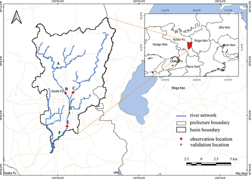
The model implementation utilizes the 5 s resolution topography data derived from the Japan Flow Direction Map (J-FlwDir) developed by Yamazaki et al. (2018). The input rainfall data are the radar and gauged composite product from the Japan Meteorological Agency (JMA) available at the spatial and temporal resolution of 1 km and 30 min, respectively. Observations for assimilation are generated from a synthetic truth model run (Section 2.5).
2.3 EnKF
2.4 Repository-based EnOI
The EnOI is a single model sub-optimal variant of the EnKF introduced by Evensen (2003). Unlike the EnKF, since only a single ensemble is integrated forward, online estimation of the model error covariance matrix is not possible for EnOI implementation. As a result, the background model error covariance matrix () and the observation error covariance matrix (𝑅) need to be defined separately. One idea is to directly use the fixed covariance matrices prepared from stationary ensembles. However, it may be desirable to use dynamic ensembles for better error characterization. Nevertheless, for both these purposes, state vector ensembles from past simulations can be used.
To prepare the background state matrix in Equation (1), it can be considered that the first ensemble is the state vector forecast obtained after the forecast stage (note that only a single model is integrated forward). The remaining ensembles are then obtained from a state vector repository which stores the vectors from past simulations. can then be calculated using Equation (2) and from an observation error parameter. The analysis is finally computed using Equation (3).
2.4.1 Repository preparation
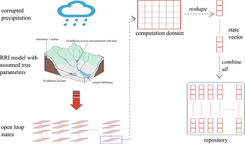
Figure 2 shows the procedure for repository preparation. First the assumed true rainfall input is perturbed by multiplicative log-normal error which is then forced into the RRI model to generate open loop states. State vectors for each ensemble at each time step are then combined together which then forms a repository. This procedure can be repeated for different flood events and for different input noise configurations to yield a collection of repositories. It should be noted that repositories can be prepared using other methodologies as well—such as through the perturbation of model parameters, or the state variables, however only the input perturbation is considered in this study for simplicity.
2.4.2 State vector sampling
After repository preparation, state vectors need to be picked from the repository in order to prepare the background state matrix. Following Toye et al. (2021), a distance-based similarity selection approach is used under the assumption that the information around the forecast may be carried by the repository states displaying similar spatial features as the forecast state. For comparing the performance of the distance-based approach, a random sampling approach is also tested.
Random sampling
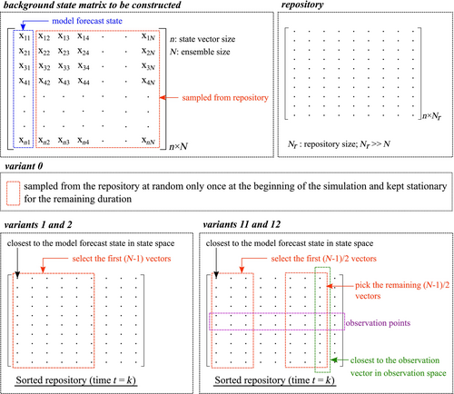
This is the simplest approach considered in the study and functions as the baseline stationary covariance matrix approach for comparison. Random sampling is chosen because there is no definitive guidance available in the literature regarding how a covariance matrix should be prepared for EnOI implementation. In this sampling method, the state vectors are sampled only once during the assimilation, that is, the ensembles in Equation (1) are stationary and chosen at random before the simulation starts. However, the first ensemble is temporally varying since this is the forecast obtained after forward integration of the model. As a result, the background error covariance matrix is actually pseudo-stationary. This approach is referred to as the EnOI variant 0 (or, EnOI_0).
Distance-based sampling
In this sampling method, the state vectors are sampled at each assimilation step, i.e., the ensembles are not stationary. Using the model forecast as the first ensemble therefore yields a fully dynamic covariance matrix.
So, at each time step , distance is computed between the forecast vector and each repository vector . The repository is then sorted in ascending order based on the computed norm (smaller norm implies more similarity between vectors and ) from which the first vectors are picked to form the background state matrix together with the model forecast. Two variants are defined based on this approach—EnOI variants 1 and 2 (or, EnOI_1 and EnOI_2) depending on whether the norm used is the l1-norm () or the l2-norm (). These norms correspond to the commonly used Manhattan norm and the Euclidean norm, respectively. Investigation with other norms is considered to be beyond the scope of this study.
This approach of using the observations along with the model forecast for state vector sampling is referred to as the EnOI variant 11 (EnOI_11) or the EnOI variant 12 (EnOI_12) depending on whether the norm used is the l1-norm or the l2-norm. Here, vectors are first sampled in the state space using Equation (5) and the remaining vectors are then sampled in the observation space using Equation (6). As a result, half of the sampled state vectors are close to the model forecast in state space while the remaining half are closer to the observations in observation space. To avoid duplicate sampling of the state vectors, already selected vectors are removed from the repository before mapping. This approach of sampling is expected to increase the background variance which may be desirable when the noise in the system is large. These different approaches of covariance matrix construction are illustrated in Figure 3.
2.5 Data assimilation experiments
Seven different flood events in the Kamo river basin (Table 1) are used to create seven repositories. Further combinations are generated by binding them.
| Event id | Event start date | Simulation duration (hours) | Event type |
|---|---|---|---|
| 1 | July 15, 2012 | 96 | Heavy rainfall |
| 2 | September 15, 2013 | 168 | Typhoon |
| 3 | August 8, 2014 | 168 | Typhoon |
| 4 | August 14, 2014 | 192 | Heavy rainfall |
| 5 | July 16, 2015 | 144 | Typhoon |
| 6 | July 5, 2018 | 192 | Typhoon |
| 7 | July 6, 2020 | 264 | Rainfall |
For assimilation experiments, the JMA truth rainfall is perturbed by spatially correlated multiplicative log-normally distributed noise (Nijssen & Lettenmaier, 2004) and fed to the RRI model with the true parameter sets. Thus produced state variables are then updated using the synthetic observations every hour.
3 RESULTS AND DISCUSSION
3.1 l1-norm vs. the l2-norm
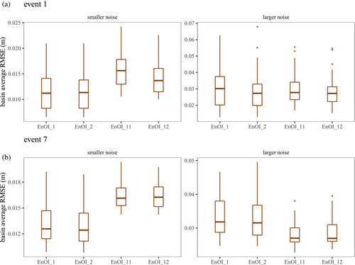
Before evaluating the performance of the EnOI approaches, l1-norm and l2-norm based state vector selection are first compared so as to reduce the number of experiments for the latter evaluations. Two repositories are prepared for the flood events from 2012 (event 1) and 2020 (event 7) and used for state vector sampling.
Figure 4 shows the basin average RMSE (m) for the two events and the two noise configurations. Here, the variants EnOI_1 and EnOI_11 use the l1-norm for distance calculation while the variants EnOI_2 and EnOI_12 use the l2-norm. Judging from the boxplots, there seems to be not much difference between using the l1-norm or the l2-norm as the RMS errors are quite similar and any superiority of one over the other is only marginal. Based on this result, the l2-norm is selected for use in the latter experiments.
3.2 Evaluation of the EnOI approaches
Figure 5 shows the comparison between the EnKF and EnOI variants, including the deterministic simulations (“Det”) in terms of the basin average RMSE for the two noise settings and two events. Forty experiments for each variant for five different repositories are combined into a box plot. For event 1, these repositories are made from (i) event 1; (ii) combination of events 2 and 5; (iii) combination of events 3, 4, and 6; (iv) combination of (ii) and (iii); and (v) all events. For event 7, the first repository is prepared from event 7 itself (instead of event 1) and the remaining are the same as those for event 1. The repository combinations (ii) and (iii) are informed by the similarity between the corresponding flood events, that is, events 2 and 5, and events 3, 4, and 6 give rise to hydrographs with similar characteristics. From the figure, it is clear that the EnKF performances are not matched by either of the EnOI variants or the deterministic simulations as the RMSE for the latter two are sometimes significantly worse than the EnKF result. This result is not surprising as the temporally varying errors are better represented in the EnKF through the multiple model ensembles which are integrated forward at each time step while the EnOI approaches try to approximate the flow dependent error from a fixed repository.

Further comparison is possible by checking the background state matrix used for covariance matrix calculation by these different approaches. Figure 6 compares the average EnKF ensemble variance calculated for the observation locations with the EnOI variances for one of the 2020 event simulations with the larger noise configuration. The repository in this case contains only the 2020 event itself. This representative plot shows that the EnOI_0 variance is generally larger than the EnKF variance. Note that since the EnOI_0 covariance matrix is pseudo-stationary, the corresponding variances are characterized by intermittent spikes instead of being constant throughout. While EnOI_2 has small variance throughout the simulation period, EnOI_12 tends to increase the spread. As this increase is not based on any diagnostic check, the latter method can wrongly increase the background variance as seen during the low flow periods. When the input noise is small (i.e., the smaller noise configuration), the EnKF variance itself becomes small, so increasing the background spread by using the observations to sample the state vectors may not be desirable in these cases, as discussed later.
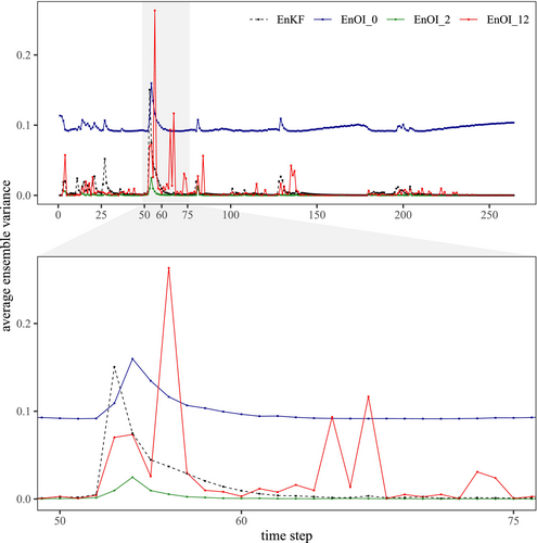
Figure 7 shows the comparison between the EnOI variants and the deterministic simulations. Box plots summarizing 40 experiments for five different repositories are shown for each variant. It is clear that variant EnOI_2 considerably reduces variability in the assimilation performance compared to EnOI_0. This is because the background spread calculated from the latter approach can be unnecessarily large due to random sampling. Bootstrapping results also suggest that the variants which use dynamic states are better than the ones with stationary states, especially for the smaller noise configuration. For larger noise configuration, even the variant EnOI_0 produces satisfactory results. However, when the error is large, instead of using the variant EnOI_2, EnOI_12, which also uses observations to sample the states, may be more suitable as the latter increases the background spread leading to slightly improved performance. In this case, increased background spread may be desirable as the model forecast is expected to be farther away from the true state due to the larger input error, and only sampling vectors similar to the forecast, while safer, may not be optimal. On the other hand, for smaller input errors, using observations to sample the model states generally produces worse results than when observations are not used for sampling.

In general, EnOI_2 tends to improve model performance compared to the deterministic simulation. However, such improvement is contingent on the repository used for sampling. For example, when the repository does not contain the simulated event itself (“repository 2,3,4,5,6” for event 1), the results from the variants using dynamic states are not always better than the corresponding deterministic simulations. A closer look indicated that, in these cases, the model spread was sometimes too large in some grids, leading to unreasonable updates to the state variables at those locations.
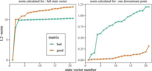
One such case is shown in Figure 8 which compares l2-norm between the model forecast and the sampled state vectors for two matrices referred to as “good” and “bad.” The “good” matrix decreases the total absolute error over the basin for the selected time step while the “bad” matrix increases this error compared to the deterministic model run. The latter is the matrix actually sampled during assimilation while the former is the one taken from a different assimilation run for comparison. Norms are calculated for two different vectors—the left panel uses the full state vector while the right one uses only one location near the basin outlet. From the plot it can be seen that for the full state vector, the sampled vectors of the “bad” matrix are closer to the model forecast (i.e., have smaller norms) than those of the “good” matrix which explains why this “bad” matrix is prepared by the algorithm and used for update during the assimilation run. However, if only one point is checked (right panel), the lines are flipped indicating that the “bad” matrix leads to a larger spread at this location compared to the “good” matrix. This may explain the large increase in error at this grid during assimilation as replacing the “bad” matrix by the “good” matrix for update reduces this error growth (Figure 9) which indicates that with a better sampling strategy, even the repository not containing the event being simulated has the potential to improve upon the deterministic simulation. However, for the current strategy, a rich repository containing multiple flood events may be required for real applications.

3.3 Computation efficiency
This section evaluates the computation efficiency of the repository-based approach. For reference, the experiments are run on a Windows desktop with Intel CPU running at 2.30GHz (40 cores and 32.0 GB of RAM). Figure 10a compares the deterministic simulation (“Det”) with the EnOI_0, EnOI_2 and EnOI_12 simulations when the repository is prepared from all seven events. The simulation durations are all normalized by the corresponding EnKF computation time. Among the three EnOI variants, EnOI_0 is the most computationally efficient as it takes only about 5% of the EnKF simulation time, which is also effectively the same as the deterministic simulation duration. This is because the only extra step in the former is the random sampling of state vectors at the beginning of the simulation. However, for EnOI_2, the normalized simulation time increases to about 40% as the state vectors are now sampled at each assimilation step after measuring the distance between the model forecast and each repository vector. EnOI_12 is the least computationally efficient as it takes about 70% of the EnKF simulation duration. The reason behind this is the additional use of observations for sampling as the norms now must be calculated twice—once in the state space and once in the observation space.
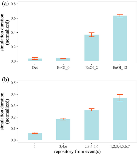
However, simulation duration for the variants EnOI_2 and EnOI_12 is significantly dependent on the repository size. Figure 10b plots the normalized simulation duration for EnOI_2 for different repository sizes (in increasing order from left to right). This increase in simulation time mainly arises during the norm calculation step as more comparison between the model forecast and the repository vectors have to be made when the repository size is increased. For example, when the repository is prepared from only the event 1, there are about 8000 vectors in the repository and the normalized simulation time is less than 10%. But for repository prepared from all seven events, this measure increases to approximately 40% as 100,000 norms (for each repository vector) need to be calculated now. A similar tendency was observed for EnOI_12, but is not shown here. Related to this, the computation time can also be expected to increase if the state vector length ( in Equations 4 and 5) is increased, such as when the basin size is large. In such a case, it may be beneficial to divide the basin into smaller sub-catchments.
3.4 Potential avenues for improvement
As seen from the results discussed until now, the EnOI approach clearly has limitations. Two of them are: (i) degraded performance at some locations and (ii) increase in computation time for a richer repository. A couple of approaches to potentially tackle these issues and improve the performance of the variant EnOI_2 are discussed in this section.
3.4.1 Use of weighted norm
The idea behind adding the weight term based on the flow accumulation number through Equations (10) and (11) is to give more importance to the downstream grids at the expense of headwater areas so that the variance at the downstream points will decrease.
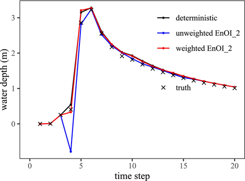
Repeating one of the experiments with negative NER discussed in the previous section by using the weighted norm, the analysis time series of water depth at one downstream location is compared to the unweighted EnOI_2 variant (Figure 11). It is clear from the figure that with the weighted variant, the degraded analysis at time step = 4 seen for the unweighted approach is avoided. However, it was found that the basin average RMSE did not change that much and the overall performance was still worse than the deterministic simulation as the errors now grew in other upstream locations (not shown) despite improvement in the downstream areas. This suggests that by appropriately weighting the norm, performance degradation at preferred locations can be prevented, but the method to reduce error over the entire basin remains to be identified. Localizing the update may be a useful strategy when the basin is large and observations are scarce.
3.4.2 Use of a sliced repository
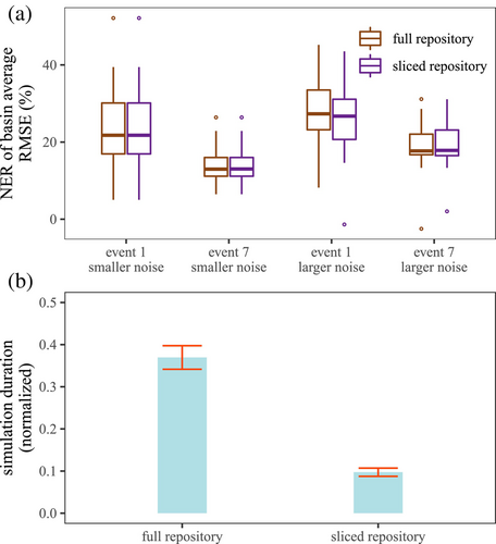
As stated earlier, a larger repository size may be required for making the EnOI approach more robust. However, a larger repository is associated with a longer computation time, rendering the methodology less attractive. To tackle this issue, an improvement to the variant EnOI_2 is considered where instead of using the full repository for norm calculation, only a portion of the repository is used. Such a portion is referred to as a “slice” and includes only those vectors which are likely to represent flow similar to the model forecast.
Before starting the simulation, norm for each repository vector is first calculated using Equation (4) (p = 2). Then at every assimilation step, before calculating the distance between the model forecast vector and the repository vectors for sampling, norm for the forecast is also calculated using the same equation. Based on the forecast norm (say, ), a range is defined where can be considered a cut-off parameter. Now only those repository vectors with norm in the range are picked to form the sliced repository. Depending on the value of the parameter , vectors corresponding to (significantly) different flow in the catchment compared to the forecast are now removed from the repository. The EnOI_2 approach can then be implemented as usual for the smaller sliced repository which can reduce the computation time.
Figure 12 compares the performance of the full repository with a sliced repository for an arbitrary of 0.2 and when the repository is prepared from all seven events. It can be seen from Figure 12a, which shows the NER of basin average RMSE calculated with respect to the deterministic simulation for two events and two noise configurations for 40 different samples each, that the performances of the full and sliced repositories are quite similar. Across the two events, almost all the experiments have the same NER measures for the two approaches for the smaller noise configuration, while approximately half of the experiments have slightly different NERs for the larger noise setting. While the maximum difference in NER across all the experiments is about 25%, the median difference is actually zero indicating that, in general, similar performance can be achieved by using only a portion of the repository. With the use of the sliced repository, the normalized computation time also reduces from approximately 40% to about 10% (Figure 12b). However, such an increase in computation efficiency is dependent on the value of the parameter as increasing it will make the approach less efficient by increasing the size of the sliced repository.
4 CONCLUSION
This study tested the idea of repository-based covariance matrix construction for assimilation of synthetic water-level observations in a distributed RRI model with the EnOI scheme. Open loop states were generated for multiple heavy precipitation events and then stored in different combinations to yield the model state repositories. While only a single model was integrated forward, the remaining ensembles were sampled from the repository to prepare the background state matrix, from which a covariance matrix could be calculated. Multiple ways of sampling were explored with the random sampling being the simplest. Other approaches involved calculating a distance measure (based on vector norm) between the model forecast (or, observation) and the repository states to select the most similar state vectors.
It was found that the distance-based sampling approach was mostly superior to sampling randomly from the repository as it led to more stable results, especially when the model error was not too large. However, the EnOI scheme was able to improve upon the deterministic simulations more consistently when the repository had information from the flood event currently being modeled. It follows then, that a richer (or, larger) repository should perform better during a real-time operation scenario. However, a larger repository meant an increase in computation time. The results showed that using a sliced repository with states closer to the forecast instead of the full repository was able to considerably reduce the simulation time. Future works should focus on developing better ways of repository construction and more efficient approaches of state vector sampling. Other methods of covariance matrix construction, beyond the repository-based approach, also need to be explored.
The results obtained in this study, especially for the distance-based approaches, are expected to be heavily dependent on the ensemble size, as the number of state vectors sampled controls the background spread. For safer results, it is desirable that the background spread be small, that is, the ensemble size is not large. However, the relationship between the ensemble size, repository properties and the optimality of the assimilation performance remains to be investigated. Further applications in real case studies are also necessary to better understand the benefits and challenges associated with using this approach. While the technique itself is general-purpose and application in different situations and catchments should be possible, actual implementation is likely to be affected by data availability, in which case satellite input data and regionalization techniques of model parameterization, among others, may have to be utilized.
ACKNOWLEDGMENTS
This work was supported by the JSPS Grants-in-Aid for Scientific Research (B) 22H01600.
Open Research
DATA AVAILABILITY STATEMENT
The data that support the findings of this study are available from the corresponding author upon reasonable request.


