Mix-and-match divestitures and merger harm

1 Introduction

Concerns of competitive harm from mergers are commonly remedied based on commitments from the merging parties either to behavioural terms, for example relating to prices or access to intellectual property, or to structural terms, which typically involve divestitures.1 Comparing these two types of remedies, Vergé 2010, p. 723) observes that there “is however a clear preference for structural remedies, because they are easier to implement and less difficult to monitor than behavioural commitments”.

Mergers involving structural remedies are the focus of this paper. Gelfand and Brannon (2016) and Cabral (2003) provide multiple examples of cases in which the merging firms propose to address merger harms by creating a new firm through the divestiture of assets. This process of seeking approval for a merger-plus-divestiture is commonly referred to as “litigating the fix”. Despite the frequent implementation of divestiture-based remedies for merger harm, theoretical foundations for these remedies have been lacking. Indeed, in FTC v. Sysco Corp., the court stated that there is a “lack of clear precedent providing an analytical framework for addressing the effectiveness of a divestiture that has been proposed to remedy an otherwise anticompetitive merger”.2

Merging firms will, in some cases, propose to divest a package of assets that includes some of each of the two merging firms' assets. Asset packages of this type are frequently referred to as mix and match. Although such a divestiture may restore the number of firms in the market to its pre-merger level, “simply finding an entity that is willing (even excited) to acquire a ‘mix and match' package of assets does not necessarily resolve the question whether competition in the relevant market will be maintained or restored”.3 For example, in United States v. Halliburton, the merging parties, oilfield services providers Halliburton and Baker Hughes, proposed to divest a substantial package of assets, but the DOJ rejected the proposed remedy as “wholly inadequate to resolve the risks to competition posed by this transaction”.4 According to Gelfand and Brannon (2016, p. 12), “the DOJ alleged that the proposed divestiture package was a hodgepodge of assets that lacked key elements and would not allow a buyer to compete effectively in the relevant businesses”.

We adapt the procurement-based framework of Loertscher and Marx (2019b) to analyse a scenario in which two firms propose to merge and simultaneously to divest production facilities from each of the merging firms to create a new firm. Consequently, the merger does not change the total number of firms in the market. For example, the S&P 500 firm Parker Hannifin Corporation acquired Clarcor in 2017, but then divested Clarcor's aviation ground fuel filtration business, paired with other Parker assets, to create a new ground fuel filtration provider. Parker retained the rest of the Clarcor businesses as well as its own aviation ground fuel filtration business.5 In reviewing a merger-plus-divestiture such as this, competition authorities may be concerned about the possibility of anticompetitive effects if the merged entity retains the superior assets and divests the others. However, articulating and substantiating these concerns is challenging because existing models and tools typically do not provide a basis for anticompetitive effects in scenarios like this. For example, Gelfand and Brannon (2016, p. 11) state: “If parties divest an entire business to eliminate any horizontal concentration (or if parties design a transaction in the first instance to avoid creating any horizontal concentration of assets), there is an argument that this precludes any concern under Section 7 of the Clayton Act”.

We show that key factors in determining the effects of a merger-plus-divestiture are whether the buyer is powerful and the extent of outside competition. A powerful buyer has the ability to hold an optimal procurement, whereas a buyer without power holds an efficient procurement (see Loertscher and Marx, 2019b). Using an optimal procurement, a powerful buyer can benefit from a transaction that creates a new lower-cost supplier, even if the transaction increases the cost of other suppliers, because a powerful buyer can use its discrimination power and monopsony power to extract better terms from the new lower-cost supplier.6 In contrast, a buyer using an efficient procurement relies on competition from higher-cost suppliers to constrain the price it must pay to the lowest-cost supplier. Thus, a buyer without power can be made worse off by a transaction that combines two suppliers to create one lower-cost and one higher-cost supplier because the buyer's payment is not determined by the lowest cost but by the costs of rivals to the lowest-cost supplier. In the absence of sufficient outside competition, the buyer without power is harmed.

Analysing coordinated effects in a procurement setting,7 Loertscher and Marx (2019a) show that a buyer is harmed by a merger-plus-divestiture that transforms two initially symmetric suppliers into two new suppliers whose distributions form a competitively neutral spread of the original distribution.8 As we show here, a merger-plus-divestiture that mixes and matches components in a way that combines the lower-cost components into one post-merger supplier and the higher-cost components into another post-merger supplier tends to be better for the buyer than a competitively neutral spread. As a result, if there is sufficient outside competition, then the merger-plus-divestitures that we consider here can benefit buyers, even in the absence of buyer power.

In related literature, Vergé (2010) considers the Cournot oligopoly model of Farrell and Shapiro (1990), in which firms are characterised by a level of assets that affects their cost function, and shows that when the pre-merger market has only three firms, then divestitures that are acceptable to the parties are never sufficient to overcome the reduction in consumer surplus from a merger. He also provides a negative result for larger oligopolies, giving conditions under which a divestiture can never successfully remedy merger harm. Vasconcelos (2010) considers merger remedies in a Cournot oligopoly consisting of four symmetric firms, where each firm has a unit of capacity. In that setup, he finds that for a three-firm merger, only a divestiture to the outside firm, rather than to a new entrant, remedies merger effects. He also finds benefits from requiring a four-firm merger to divest two units to create a rival. Cabral (2003) analyses the effects of a merger in a spatially differentiated oligopoly where the industry is assumed to be at a free-entry equilibrium, both before and after the merger. He shows that voluntary asset sales by the merging parties reduce consumer surplus by deterring entry.

Some papers have raised concerns that certain divestitures can exacerbate concerns of coordinated effects, for example if the firms in a market following a merger-plus-divestiture are more symmetric with one another than before the transaction (see Compte et al., 2002; Vasconcelos, 2005; Loertscher and Marx, 2019a). Our focus here is on unilateral rather than coordinated effects.

In Section 2, we describe the setup. In Section 3, we analyse the effects of a merger-plus-divestiture and how those effects relate to buyer power and the degree of outside competition. Section 4 concludes.

2 Setup

We adapt the setup of Loertscher and Marx (2019b) to allow for the possibility of mix-and-match divestitures by introducing intermediate products that suppliers must combine to produce a final product, but that can potentially be divested separately.

We assume that each supplier combines two intermediate products, A and B. The buyer has value zero for the intermediate products individually and has value v > 0 for one unit of the finished good. This setup can equivalently be thought of as reflecting an environment in which the buyer does not have the capability to combine the intermediate products to produce the final good or one in which the buyer simply has a strong preference for one-stop shopping, for example because of a desire for clear liability in case of disputes after contracting.

Let be the pre-merger set of suppliers, where suppliers 1 and 2 are the merging suppliers. We assume that each supplier i draws its total cost for the finished good from a continuously differentiable distribution . We assume that for all , is defined on support [0, ∞) with a density that is positive on the interior of the support and has finite expectation.9 Each supplier's cost is its own private information. All agents are risk neutral and have quasilinear payoffs, so that, for example, if supplier i's expected payoff when its cost is , the probability that it trades is and its expected transfer is is .

We assume that the total cost for the finished good is the sum of the costs of producing the two intermediate products. That is, for each , we let there be continuously differentiable distribution functions and , also with support [0, ∞) and densities and that are positive on the interior of the support, such that is the distribution of the sum of independent draws from distributions and ; that is, is the convolution of and :

In the absence of divestitures, the merged entity draws its cost from , which is the distribution of the minimum of the cost draws of suppliers 1 and 2. However, if the merged entity divests supplier 2's production facility of A and supplier 1's production facility of B, then the merged entity draws its cost from the convolution of and , which we denote , and the newly created supplier based on the divested assets draws its cost from the convolution of and , denoted . We focus on this divestiture possibility because it is the one that leaves the market with the same number of suppliers before and after the merger.

For purposes of illustration, we work with cost distributions that are Gamma distributions. A Gamma distribution is defined by two parameters, a shape parameter and a scale parameter, and is approximately normal for a shape parameter of 10 or larger. The mean of a Gamma distribution is equal to the product of its shape and scale parameters, so in our illustrations, which all assume a scale parameter equal to one (i.e., a “standard” Gamma distribution), the shape parameter is the mean. For modelling divestitures, the standard Gamma distribution has the particularly convenient feature that the convolution of two standard Gamma distributions with means s and is a standard Gamma distribution with mean .

As mentioned, a buyer without buyer power purchases using a competitive procurement such as a descending-price auction with reserve v that allows it to purchase from the lowest-cost supplier at a price equal to the minimum of v and the second-lowest cost. A buyer with buyer power purchases using an optimal procurement. In the optimal procurement, the buyer purchases from the supplier with the lowest virtual cost, if and only if that virtual cost is less than or equal to the buyer's value v. For the pre-merger suppliers, the virtual cost of supplier i when its cost draw is is , and the virtual cost of the merged entity when its cost is c is . Analogously, the virtual cost of a supplier constructed from supplier i's production of A and supplier j's production of B is , where and 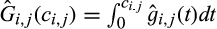. When a powerful buyer makes a purchase, it pays the supplier with the lowest virtual cost an amount equal to the worst type for the winning supplier that would still have resulted in trade with that supplier. This is commonly referred to as the supplier's threshold type.

We make use of the revelation principle which says that we can focus without loss of generality on direct mechanisms 〈q, m〉 that ask each supplier to report its type and, as a function of reports c, determines an allocation q and transfers m that respect suppliers' incentive compatibility and individual rational constraints.10 Moreover, by the payoff (or revenue) equivalence theorem, once the allocation rule is determined, the expected transfers are pinned down up to a constant, which in our case is zero.11 Therefore, the main focus in the analysis that follows is on the allocation rules.

Before the merger, let be an allocation rule that maps the vector of types c onto .12 The allocation rule has the interpretation of specifying, for each type profile, the probability with which each supplier trades with the buyer. Given the allocation rule, standard mechanism design arguments imply that the buyer's expected surplus in the pre-merger market is

()

Following a merger with no divestiture, expected buyer surplus is

()

where is the probability of trade with the merged entity and the allocation rule is the allocation rule that maps the vector of types onto .

Following a merger-plus-divestiture in which supplier i's product A is combined with supplier j's product B (where i, j ∈ {1, 2} with i ≠ j), we denote the thus created firms by i, j and j, i, respectively. An allocation rule now maps reported costs onto . Accordingly, expected buyer surplus following a merger-plus-divestiture is

()

3 Results

We now analyse the effects of a merger-plus-divestiture. We focus on the case in which each merging supplier has an advantage in the production of one of the inputs in the sense of first-order stochastic dominance (FOSD). In particular, when comparing two cost distributions, we say that one cost distribution is “better” than the other if it is first-order stochastically dominated by the other and “worse” if it first-order stochastically dominates the other. In what follows, we assume that between the two merging suppliers, supplier 1 has a relative advantage in producing input A in the sense that is better than and that supplier 2 has a relative advantage in producing input B in the sense that is better than . Thus, because sums of independent random variables preserve stochastic ordering, the convolution of and is better than the convolution of and (Aubrun and Nechita, 2009).

We consider a merger-plus-divestiture in which the merging suppliers divest the weaker of each input pair. That is, the merged entity divests supplier 1's B production and supplier 2's A production, selling them to a common acquirer (who will then become a new supplier).13 Thus, the merged entity retains supplier 1's superior A production and supplier 2's superior B production, while divesting the lesser assets. Such a transaction replaces the merging suppliers 1 and 2 with two different suppliers: supplier 2, 1, whose cost distribution is worse than the distributions of the merging suppliers, and supplier 1, 2, whose cost distribution is better than the distributions of the merging suppliers. That means that in the post-merger market, it is more likely that some supplier will have a cost less than, say, v, but the expected value of second-lowest cost may be higher, depending on the extent of outside competition.

3.1 Effects of the distribution of the second-lowest cost

For a buyer without power, having the lowest cost less than v does not contribute to surplus unless the second-lowest cost is also less than v because when only one cost is less than v, the buyer without power pays v and so has zero surplus. Thus, for a buyer without power, the effect of a merger-plus-divestiture depends on the effect on the distribution of the second-lowest cost. In contrast, a powerful buyer can benefit from a merger-plus-divestiture even if the distribution of the second-lowest cost worsens.

Proposition 1 establishes conditions under which a merger-plus-divestiture is anticompetitive and conditions under which it is procompetitive.

Proposition 1.A merger-plus-divestiture that results in a worse distribution of the second-lowest cost harms a buyer without power but can benefit a buyer with power. A merger-plus-divestiture that results in a better distribution of the second-lowest cost benefits a buyer without power.

Proof.See Appendix A.

As shown in Proposition 1, even though a merger-plus-divestiture does not change the number of suppliers in the market, a buyer without power is harmed if a merger-plus-divestiture results in a worse distribution of the second-lowest cost. In the absence of buyer power, the buyer uses competition to police the price that it pays to the winning supplier. A merger-plus-divestiture that worsens the distribution of the second-lowest cost relaxes that pricing discipline. In contrast, a powerful buyer can also discipline prices through its use of its monopsony power by applying reserve prices and its discrimination power by handicapping stronger suppliers, and so a powerful buyer can potentially take advantage of a merger-plus-divestiture that increases the second-lowest cost, as long as it reduces the lowest cost.

Table 1 provides an example of a merger-plus-divestiture that is procompetitive when the buyer is powerful but anticompetitive when the buyer does not have power, where we measure the competitiveness of the transaction by its effect on buyer surplus. In the example of Table 1, the expected surplus of a buyer without power decreases 28% as a result of a merger-plus-divestiture, while the expected surplus of a buyer with power increases 24% from the same transaction.

Table 1. Effects of a merger-plus-divestiture when n = 2 and , , and are standard Gamma distributions with corresponding means and and v = 12

	Buyer power
	Without	With
Pre-merger expected buyer surplus	5.79	6.24
Post-merger + divestiture expected buyer surplus	4.14	7.75
Change in expected buyer surplus	−28%	24%

The results of Proposition 1 extend to mergers (or consolidations) among any number of suppliers. To see this, suppose that the final good is produced from the combination of k components. Then there may be an incentive for a merger involving as many as k suppliers, so that a single supplier can be created that takes the best from each. Therefore, assume that k suppliers merge and then divest assets to produce one supplier whose total cost is drawn from the convolution of the best distributions for each of the k individual components and that the k−1 other suppliers have costs constructed from the various combinations of the remaining components. Then the merger-plus-divestiture again reduces the expected surplus of a buyer without power if it worsens the distribution of the second-lowest cost and increases a buyer's expected surplus if it improves the distribution of the second-lowest cost.

To refine the result of Proposition 1, consider the case of n = 2 and assume that , , , and are standard Gamma distributions with corresponding means This implies that supplier 1's product A and supplier 2's product B are similarly low cost, while the complementary products are similarly high cost. Then the distribution of the second-lowest pre-merger cost is and the distribution of the second-lowest post-merger cost is . Thus, for a buyer without power, the change in expected buyer surplus as a result of the merger-plus-divestiture is

()

which, as we show in the next proposition, is always negative for a sufficiently small difference between and .

Proposition 2.A buyer without power is harmed by a merger-plus-divestiture when there are two pre-merger suppliers and they draw their costs from standard Gamma distributions with integer means , where is sufficiently small.

Proof.See Appendix A.

We illustrate Proposition 2 in Figure 1. Figure 1a shows three standard Gamma distributions with means 2, 5 and 8 which correspond to the possible convolutions of pairs of distributions with means 1 and 4. Figure 1b shows that the change in the buyer's expected surplus, given by Equation (4) is negative for a buyer without power for a range of distributional parameters, indicating that a merger-plus-divestiture harms a buyer without power. However, for a buyer with power, the change in expected surplus is positive for the same parameters.

As reflected in Figure 1b, as s increases from 1, a powerful buyer's expected payoff increases and then levels off. As increases, the pre-merger and post-merger surpluses of a powerful buyer decrease, but as s grows large, the pre-merger expected payoff approaches zero while the post-merger surplus approaches a positive constant because the new supplier with the better cost distribution likely trades at its reserve price. In contrast, for a buyer without power, as s increases above 1, the post-merger payoff decreases more quickly than the pre-merger payoff (reflecting the worsening of the distribution of the second lowest), but eventually as s grows large, the buyer pays its reserve of v with high probability both pre-merger and post-merger, so the change in the buyer's expected payoff goes to zero.

Although the analytic result of Proposition 2 requires that be sufficiently small, the example of Figure 1b shows that Equation (4) is negative not only for close to but apparently for all , suggesting that the result holds more generally.

3.2 Effects of the distribution of the lowest cost

Propositions 1 and 2 are based on the effect of a merger-plus-divestiture on the distribution of the second-lowest cost. In this subsection, we focus on the effect of a merger-plus-divestiture on the distribution of the lowest cost. As we show, if a merger-plus-divestiture results in a better distribution of the lowest cost, then a buyer without power benefits as long as there is sufficient outside competition.

To describe the effects of a merger-plus-divestiture on the distribution of the lowest cost of the pre-merger merging suppliers versus the newly created suppliers following a merger-plus-divestiture, we use the notion of a neutral for rivals spread (see Loertscher and Marx, 2019a). A pair of distributions is said to be a neutral for rivals spread of G if is better than G and is worse than G in an FOSD sense, and if the distribution of the minimum of two draws from G, given by , is the same as the distribution of the minimum of one draw from and one draw from , given by . That is: for all c ≥ 0,

and

Loertscher and Marx 2019a, Proposition 9) show that a buyer without power is harmed by a merger-plus-divestiture that creates a neutral for rivals spread. However, as we show below, a merger-plus-divestiture that mixes and matches components in a way that combines the lower-cost components into one post-merger supplier and the higher-cost components into another is in many cases better than a neutral for rivals spread. Moreover, if a merger-plus-divestiture produces new suppliers that have a better distribution for the minimum of their costs than the merging suppliers, then a buyer without power benefits as long as there is sufficient outside competition.

Proposition 3.Given sufficiently many symmetric outside suppliers, a buyer without power benefits from a merger-plus-divestiture if the distribution of the minimum cost of suppliers 1,2 and 2,1 is better than the distribution of the minimum cost of suppliers 1 and 2. That is, assuming n−2 symmetric outside suppliers, there exists such that for all , the buyer's expected surplus increases following the merger-plus-divestiture if for all c ≥ 0,

()

with a strict inequality for an open subset of the support.

Proof.See Appendix A.

Proposition 3 provides conditions under which a buyer without power benefits from a merger-plus-divestiture, and those conditions are satisfied under the distributional assumptions of Proposition 4, which gives us the following proposition:

Proposition 4.Given a sufficiently large number of outside suppliers, a buyer without power benefits from a merger-plus-divestiture when the merging suppliers draw their costs from the standard Gamma distribution with integer means , where is sufficiently small.

Proof.See Appendix A.

To illustrate Propositions 3 and 4, consider the example in which supplier 1 and supplier 2 each has a pre-merger average cost of 10. Supplier 1 has a relative advantage in producing input A, which has an average cost of 4, while the average cost of input B is 6. Supplier 2 has a relative advantage in producing input B, whose average cost is 4, while its cost for producing input A is 6. The suppliers propose to divest supplier 1's production facility for input B and supplier 2's production facility for input A, selling them to a common acquirer, and to retain the superior production technology of supplier 1 for A and the superior production technology of supplier 2 for B. Suppose all of the pre-merger distributions are standard Gamma distributions. With the proposed divestiture, the merged entity would have a cost distribution that is also a standard Gamma distribution but with mean 8, and the newly created supplier from the divestiture would have a cost distribution that is a standard Gamma distribution with mean 12. Assume that outside suppliers, if there are any, draw their costs from a standard Gamma distribution with mean 12. This implies that each outside supplier has the same production technology as the newly created supplier that emerged from the divestiture.

The pre-merger and post-merger buyer surplus are depicted in Figure 2, both without and with buyer power, and for a range of numbers of outside suppliers.

As shown in Proposition 2, a merger-plus-divestiture in this setting is anticompetitive for a buyer without power when there is no outside competition. This is reflected in Figure 2a, which shows that the buyer without power is harmed when there are few outside suppliers. The worsening of the cost distribution of one of the post-merger suppliers means that a buyer without power pays more in the post-merger market when it relies on the supplier with the worse cost distribution to determine the price. When there are many outside suppliers, the worsening of the cost distribution for one supplier is less relevant, and, as shown in Proposition 4, the benefit of having a supplier with a better cost distribution eventually dominates in the setting of Figure 2. That is illustrated in Figure 2a by the increase in the post-merger buyer surplus above the pre-merger buyer surplus as the number of outside suppliers increases.

In contrast, when the buyer is powerful, as shown in Figure 2b, the merger-plus-divestiture is procompetitive, increasing the expected surplus to the buyer, even when there is no outside competition. The merger-plus-divestiture creates a supplier that has a better cost distribution than any supplier in the pre-merger market, and a powerful buyer benefits from that.

Thus, a merger-plus-divestiture is a concern for a buyer without power when there is little outside competition but benefits the buyer regardless of power when there is sufficient outside competition. Intuitively, the new lower-cost supplier created by the merger-plus-divestiture only benefits a supplier without power if competition from other suppliers can then drive prices towards that new lower cost.

4 Conclusion

In this paper, we focus on the effects on a buyer as the result of a merger-plus-divestiture among the firms that supply that buyer. Our model is one of incomplete information, where suppliers costs are their own private information. It extends the procurement model of Loertscher and Marx (2019b) to accommodate divestiture.

Although a powerful buyer can benefit from a divestiture that creates a lower-cost supplier, even if it causes costs for another supplier to increase, a buyer without power is harmed in the absence of sufficient outside competition. In particular, without power, a buyer without sufficient competitive alternatives is harmed by a divestiture that creates a lower-cost supplier at the expense of increasing the costs of another supplier. The intuition for this is that a powerful buyer benefits from the opportunity to deal aggressively with a lower-cost supplier, but a buyer without power is harmed if there is a weakening of the competitive constraint on the lowest-cost supplier.

While the model of this paper assumes a single buyer, extensions could allow multiple buyers with varying power as in the analysis of varying sizes of grocery stores in Igami (2011). In other extensions, one could incorporate cost synergies, or the loss of cost synergies from the mix and match process. As shown in Igami and Uetake (2019) for the hard disk drive industry, the effects of synergies can be significant.

References

- 1 See Lévêque and Howard (2003) for an overview of remedies used in the United States and the European Union and Duso et al. (2006) for empirical analysis of the effects of remedies. See also the U.S. Department of Justice's “The Antitrust Division Policy Guide to Merger Remedies”, June 2011, available at https://www.justice.gov/sites/default/files/atr/legacy/2011/06/17/272350.pdf.
- 2 FTC v. Sysco, 113 F. Supp. 3d 1, 72 (D.D.C. 2015).
- 3 U.S. Federal Trade Commission, “Frequently Asked Questions About Merger Consent Order Provisions”, Q.21 and Q.22, available at https://www.ftc.gov/tips-advice/competition-guidance/guide-antitrust-laws/mergers/merger-faq#The%20Assets%20To%20Be%20Divested.
- 4 Complaint, United States v. Halliburton, No. 16-cv-00233_UNA (D.D.C. 2016), p. 2.
- 5 “Parker Completes Divestiture of Facet Filtration Business to Filtration Group Corporation”, 30 April 2018, Globe Newswire, available at https://globenewswire.com/news-release/2018/04/30/1489935/0/en/Parker-Completes-Divestiture-of-Facet-Filtration-Business-to-Filtration-Group-Corporation.html.
- 6 Using terminology frequently applied in antitrust, Loertscher and Marx (2019b) call the ability to set a binding reserve price (i.e., a reserve price that sometimes prevents efficient trade from occurring) monopsony power and the ability to discriminate among ex ante heterogeneous suppliers bargaining power. In light of the fact that bargaining power has other connotations and, in particular, is meaningful even in bilateral bargaining, calling the latter discrimination power, as we do here, seems preferable.
- 7 For an analysis of coordinated effects in a repeated oligopoly setting, see, for example, Compte et al. (2002), Vasconcelos (2005) and Bos and Harrington (2010).
- 8 As defined in Loertscher and Marx (2019a), two distributions form a competitively neutral spread of an initial distribution if one distribution is better than the initial distribution and the other is worse in a first-order stochastic dominance sense, but the distribution of the minimum of two draws, one from each, is the same as the distribution of the minimum of two draws from the initial distribution.
- 9 As shown in Giannakopoulos (2015), the assumption of finite expectation is sufficient for the usual mechanism design arguments of Myerson (1981) to go through when distributions have unbounded upper bound of support.
- 10 See, for example, Myerson (1981) or Krishna (2002).
- 11 Again, see, for example, Myerson (1981) or Krishna (2002).
- 12 In an auction to sell one item, feasibility would require that the quantity vector be an element of the n-dimensional simplex because the seller cannot sell more than the one item. In contrast, in a procurement auction, the buyer could purchase more than one unit even if it has demand for only one unit. Therefore, in a procurement, the restriction to the simplex is an implication of optimality rather than feasibility.
- 13 For an analogous analysis of divestiture by a vertically integrated buyer, see Loertscher and Riordan (2019).
- 14 A function
is absolutely continuous if for all ɛ > 0 there exists δ > 0 such that whenever a finite sequence of pairwise disjoint sub-intervals
of [v, v] satisfies
, then
. One can show that absolute continuity on compact interval [a, b] implies that h has a derivative
almost everywhere, the derivative is Lebesgue integrable, and that