Necessary changes to improve animal models
Summary
Animal models evolved from sire models and inherited some issues that affected sire models. Those issues include definition and treatment of contemporary groups, accounting for time trends and dealing with animals having unknown parents. The assumptions and limitations of the animal model need to be kept in mind. This review of the animal model will discuss the issues and will recommend enhancements to animal models for future applications.
1 INTRODUCTION
 (1)
(1)where
- yijklm was first lactation 305-day milk yield of daughter m of sire l belonging to genetic group k making a record in year-season of calving i and herd-year-season j;
- YSi was a fixed year–season of calving effect to account for time trends in the data;
- HYSij was a random herd-year-season (HYS) of first calving contemporary group;
- Gk was a fixed sire genetic group, defined by the year of sampling and AI ownership;
- Skl was a random sire effect within genetic group; and
- eijklm was a random residual effect.
In matrix notation, let
- y be the vector of first lactation milk yields,
- b be the vector of fixed year–season effects,
- h be the vector of random herd-year-season effects,
- g be the vector of fixed genetic group effects,
- s be the vector of random sire transmitting abilities, and
- e be the vector of random residuals,
 (2)
(2)where X, W, Q and Z are design matrices relating observations to the factors in the model.
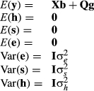
The assumptions of this model were
- Sires were unrelated to each other.
- Sires were mated randomly to dams.
- Progeny were a random sample of daughters.
- Daughters of sires were randomly distributed across herd-year-seasons.
- Milk yields were adjusted perfectly for age and month of calving.
The limitations were
- Sires were related to each other.
- Semen prices varied among sires depending on the background of the bull. Sires were not randomly mated to dams in the population.
- Daughters of higher priced bulls tended to be associated with elite herds that supposedly had better environments for cows.
- The age and month of calving adjustment factors were not without errors.
- Only first lactation records were used.
- Cows were not evaluated.
2 FIXED VERSUS RANDOM FACTORS
Most statistics books in 1970 would define a fixed factor as one with relatively few levels, such as age groups, treatments, diets and years, of which differences among the levels were to be estimated. If the experiment was to be repeated, then the same levels of ages, treatments or diets might appear again, and their estimated differences would be expected to be consistent between the two samples. However, year effects would differ in a repeated sampling approach because time does not stand still and years do not repeat themselves. In the proposed model above, year-seasons were considered to be a fixed factor because there were a limited number of years and seasons per year in the data.
A random factor, on the other hand, would have many levels, large enough to be considered infinite and large enough to be viewed as being randomly sampled from an infinite population, such as sires or herd-year-seasons. If the study was repeated, then the sires and herd-year-seasons would be completely new, a different random sample. In animal breeding situations, studies are not repeated, but instead new sires and new herd-year-seasons are constantly being generated based partly on the composition of previous samples and thus only occur once. Sire effects were considered a random factor even though the number of sires was less than 1,500 for Holsteins, which is significantly less than infinite. Herd-year-season effects were also a random factor having around 100,000 levels.
The distinction between fixed and random factors was also based on how the results were to be interpreted. With a fixed factor, interest was on the estimated differences between levels of that factor for those specific levels of the factor. For example, if there were two diets involving different components, then the researcher would be interested in the different impacts of those diets on milk production or growth. There could be 50 other diets that could be compared, but the experiment was only for those two specific diets. With a random factor, the researcher would be more interested in the variation of effects of levels of random factors on milk production or growth, and not in any specific levels of the random factor. Herd-year-season effects might account for 10% of the variation in milk yields across the country. This fact was more important than the specific difference between 2 year-seasons within one herd. In genetic evaluation, data are being analysed, and researchers are interested in the realized values of levels of a random sire factor.
Levels of random factors occur outside the control of the researcher. Researchers do not decide which herd-year-seasons will have cows calving and certainly do not control the effect of that herd-year-season on the yields of cows. The researcher also does not control the number of herd-year-seasons that will be, or where they will be. On the other hand, researchers do decide which diets will be compared, in which herds, and which animals, and thus, diets are a fixed factor. Basically, any experiment in a research environment will have mostly fixed factors in the model, whereas data collected from livestock producers will have more random factors influencing the observations that the researcher has not been able to control.
Determining whether a factor is fixed or random undergoes many shades of grey in practice. In the end, the researcher makes the decision based on experience and tradition in that field of study. For a complete discussion see LaMotte(1983).
3 BETTER SIRES IN BETTER HERDS
Before the Northeast AI Sire Comparison became public, the industry in the northeast believed that the better sires were used in the better herds thus creating a bias in sire estimated transmitting abilities. Henderson had a theory about different kinds of selection bias and how to account for them which he had taught in his graduate course at Cornell since 1965, but did not publish until 1975.
To illustrate the problem, consider the progeny data in Table 1 representing 1 year–season, three herds and four sires ignoring genetic groups in this example.
| Herds | (nij,yij.) | Herd totals | |||
|---|---|---|---|---|---|
| Sires | |||||
| 1 | 2 | 3 | 4 | ||
| 1 | (9,270) | (16,432) | (0,0) | (0,0) | (25,702) |
| 2 | (1,27) | (3,72) | (5,85) | (1,12) | (10,196) |
| 3 | 0 | (1,21) | (25,350) | (39,351) | (65,722) |
| Sire totals | (10,297) | (20,525) | (30,435) | (40,363) | (100,1620) |
Note that sires 1 and 2 have most of their progeny in herds 1 and 2, and sires 3 and 4 have most of their progeny in herds 2 and 3. In creating the data, sires 1 and 2 had positive true breeding values, and sires 3 and 4 had negative true breeding values. Also, herd 1 true value was better than herd 2 and herd 3; herd 2 true value was better than herd 3. Thus, the better sires in better herds selection bias were constructed. In real life, of course, this cannot be done, but industry personnel believed that this bias was occurring.
 (3)
(3)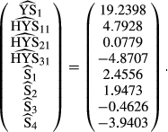
The sire solutions are presumably biased because of the selection bias issue.
 (4)
(4) describes selection differentials and θ is a vector of the estimates of selection bias, kh is the ratio of residual to herd-year-season variances, and ks is the ratio of residual to sire variances. Unfortunately, Henderson (1975) or Henderson (1984) did not give any hints about creating an appropriate L, only that one exists.
 were attempted. Here, u is taken to be h, the herd-year-season random effects. A selection differential expresses a function that describes the difference between one HYS from the other HYS. One possible matrix is

This matrix says that HYS11 is better than the average of HYS21 and HYS31 (first row of  ), and that HYS21 is better than HYS31, and HYS31 is not better than any HYS.
In Henderson (1984), he makes  , which states that each HYS is unique. The solutions from the two attempts and the original solutions to the MMEs are in Table 2.
 , and MMEs using
| Effects | Original | With  |
With  |
|---|---|---|---|
| YS1 | 19.2398 | 20.6401 | 19.5479 |
| HYS11 | 4.7928 | 6.6348 | 7.7269 |
| HYS21 | 0.0779 | −1.4166 | −0.3245 |
| HYS31 | −4.8707 | −8.3010 | −7.2089 |
| S1 | 2.4556 | 1.2921 | 1.2921 |
| S2 | 1.9473 | 0.5312 | 0.5312 |
| S3 | −0.4626 | 0.6757 | 0.6757 |
| S4 | −3.9403 | −2.4990 | −2.4990 |
| θ1 | 66.3476 | 77.2691 | |
| θ2 | 19.0076 | −3.2447 | |
| θ3 | −30.8289 | −72.0889 |
- MMEs, mixed model equations.
 , and that estimable functions of the other effects are also identical. For example, the solution for
  is the same in the last two columns. Several other
  matrices were constructed and tried, and all gave the same solutions for sire effects. Henderson likely tried many
  matrices too and came to the conclusion that the exact structure of
  did not matter. Thus, let
  , then the above equations reduce to

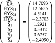
The sire solutions are the same as those in the last two columns of Table 2, and YS1 + HYS11 is also identical. Thus, treating random HYS as a fixed factor removes the selection bias due to better sires being used in the better herds. It seems incredulous that seemingly any  matrix can be used, as long as there are three independent rows.
Hence, Henderson used model (2) with random HYS effects, that is contemporary groups (CG), treated as fixed in the first official run of the northeast AI sire comparison. Ever since, random HYS effects have been treated as a fixed factor in sire and animal models, except in a few rare cases, but always considered to be a random factor. There has never been a study on the amount of bias that supposedly existed, nor on the increase in prediction error variances as a result of making HYS effects fixed.
Thompson (1979) argued that  was not well defined, and therefore, Henderson's selection bias theory was not sound. Gianola, Im, and Fernando (1988) gave Bayesian arguments against the concept of repeated sampling underlying the assumptions of Henderson's theory to derive the modified MMEs. Therefore, if Henderson's selection bias theory is unsound, then have animal breeders made a mistake in treating random HYS as a fixed factor? How much genetic change has been lost as a result, if any?
 (5)
(5)where W, Q and Z are design matrices relating observations to the factors in the model. Note that h is now treated as fixed effects in the model and that year-season effects, (Xb), were totally confounded with herd-year-seasons and thus were not estimable in this model, and therefore, removed.

In the northeast United States, HYS subclasses were fairly large, but in some European countries, there were many HYS with fewer than five animals. Any HYS with all daughters from only one bull did not contribute any information to sire evaluations. Not much data were lost in the northeast United States, but in Europe, there were many more HYS with only one or two cows, which were lost when random HYS effects were treated as a fixed factor.
The other assumptions and limitations were as with the initial model (2). The problems of sires being related, and not being randomly mated to dams were probably much more significant in their effects on estimated transmitting abilities than the problem of non-random association of sires with herd-year-season effects, but were largely ignored.
The modified model (5) is the one that every country tried to adopt during the 1970s. I gave courses in Sweden and Switzerland in 1976 on how to use Henderson's programs, and those notes still pop up when I visit other countries (Schaeffer, 1976). Thus, model (5) became the accepted practice even if the bias that was present in the northeast United States did not exist in other countries or situations. For example, sire models used in swine or sheep, where artificial insemination was not prevalent and where progeny group sizes were not large, probably had no selection bias that needed removal. CGs could have remained a random factor in those models without issue.
4 SIRES RELATED

The sire model continued to be employed for sire evaluation until 1988. By 1988, computer hardware and computing techniques (such as iteration on data, Schaeffer & Kennedy, 1986) had improved to make animal models feasible (Jamrozik & Schaeffer, 1988; Wiggans & Misztal, 1987).
In summary, the problems with sire models were
- Sires were not randomly mated to dams.
- Having enough bulls in each genetic group.
- Only first lactations of cows were used.
- No cow evaluations were produced.
- HYS with all cows being daughters of the same bull were useless.
Problems motivate changes for the future, and the problems of the sire model motivated change to an animal model.
5 ANIMAL MODELS
Papers by Thompson (1979) and Gianola et al. (1988) criticized the selection bias theories of Henderson (1975) and effectively stopped all future discussion about Henderson's selection bias theories. The fact that  selection theory was deemed incorrect, meant that the sire model with random HYS treated as a fixed factor might not be appropriate because it was based on unsound theory. However, even in 2018, random HYS effects are frequently treated as a fixed factor for animal models.
Several papers have argued the merits of fixed or random CGs (Ugarte, Alenda, & Carabano, 1992; Van Vleck, 1987; and Visscher & Goddard, 1993). However, there is no question that HYS, or CGs, are a random factor in the sense of traditional statistics teachings, and in terms of field data used in animal breeding work. The argument should be does treating HYS as a fixed factor remove the selection bias of the better sires being associated with the better HYS.
If contemporary group size is large (e.g., 20 or more individuals), then there is little difference in analyses if they are a fixed or random factor. Keep in mind, it is not sufficient to make CGs random by adding Ikh to the diagonals of  , but it is also necessary to add Xb, phenotypic time trends, as a fixed factor, back into the model, otherwise biases will occur. Genetic trends are estimated through the A matrix as long as pedigrees are complete and can trace animals back to the base generation, and all data are included (Kennedy, Schaeffer, & Sorensen, 1988).
6 CONTEMPORARY GROUPS
Contemporary groups are usually considered to be a nuisance factor in the model. A factor that causes variation in the observations which must be taken into account. This interpretation is the same whether CGs are a fixed or random factor. If there is any interest in the actual estimates of CG effects, then commonly differences among CG are considered or the variation of CG effects as a percentage of the total phenotypic variance. In some milk recording schemes, the estimates of CG effects are provided back to herdowners through time plots, which the owner may relate to past feeding practices or environmental changes.
Contemporary groups should always be a random factor in animal models and sire models, because this is a factor not controlled by the researcher, is a factor usually with the most levels (considered large enough to be infinite); under repeated sampling concepts would be vastly different between samples; and there is no valid existing theory that implies they should be treated as fixed.
Contemporary groups are used to identify a group of animals that are
- The same gender,
- Born in the same year-month,
- Raised in the same herd, pen, cage, barn or field and
- Received the same feed and management care.
As animals grow and enter different phases of their life, they may change to different CGs. Instead of being born in the same year-month, they may be born in the same year-season (a group of 3 or 4 months combined).
The animals which will constitute a future CG is not known ahead of time. One might know which cows will give birth to a calf, but it is not known which calves will survive parturition, and it is not known which will be male or female (unless sexed semen is used, which changes the probabilities). One does not know what future environment or feed quality will exist for a future CGs. Thus, the future CG effect has an expectation of 0 with a standard deviation of σh. By definition and manner of creation, CGs are a random factor for any linear model analysis.
7 THE MODEL
There are a few elements which should be present in all animal models. They are
- Fixed time period effects,
- Random contemporary group effects,
- Random animal additive genetic effects and
- Phantom parent groups because there are always animals with unknown parents.
 (6)
(6)- b is a vector of fixed effects (such as age, year, gender, farm, cage and diet) that affect the trait of interest, and is not genetic in origin,
- u is a vector of random factors (such as CGs and others),
- p is a vector of permanent environmental effects,
- aw are animals with records, and ao are animals without records in y, but which are related to animals in aw,
- e is a vector of residual errors,
- X, W and Z are design matrices relating observations in y to factors in the model.
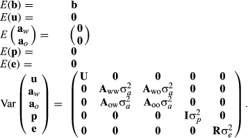

for i going from 1 to the number of other random factors in the model, and R is usually diagonal, but there can be different values on the diagonals depending on the situation. Often all of the diagonals are the same, so that  .
.

Some of the assumptions of an animal model are
- Random factors follow normal distributions.
- Progeny of sire–dam pairs are random from amongst all possible progeny of that pair.
- Selective matings of sires to dams are taken into account through the relationship matrix (Kennedy et al., 1988).
- Animals are randomly dispersed across levels of fixed factors.
- Observations are taken on either males or females, but if taken on both sexes, then the assumption is that parents would rank the same if based only on one gender or the other.
- No preferential treatment has been given to individuals or groups of individuals.
- Data should not be a selected subset of all possible animals.
- Every animal is able to express their full genetic potential without restraint from other individuals within their CGs.
- Animals can be traced to a common base population of unselected and randomly mating individuals.
Preferential treatment is where the environment of one or a few animals is artificially enhanced relative to the majority of individuals in a CG. Some animals are frequently separated from their contemporaries for better care, but when the supervisor is visiting the herd, the animals are temporarily merged with the other contemporaries. The special treatment is usually not recorded in the data. There is no known statistical procedure for accounting for preferential treatment, except for removal of records of preferentially treated animals.
In the era of genomics, assumptions 2 and 7 are violated today with an animal model (Tyriseva et al., 2018). When embryos are genotyped, and the “poorer” ones are discarded, then data are being selected because the poorer ones are not included in creating a genomic relationship matrix, and of course, do not ever have progeny or make a phenotype and are in no way recorded or identified in any database. The validity of an animal model (or single-step GBLUP) is thrown entirely into question.
There should never be a need to pre-adjust observations for any factor. With today's hardware and software, these factors can be placed in the animal model and solved simultaneously with the other factors of the model. Any fixed factor in any animal model may need an interaction with time. For example, in dairy cattle, differences between age groups or months of calving can change over the years. An interaction of age and month of calving with years of calving (5-year periods maybe) is needed in the animal model. Suppose in 1973, the difference between 24 months of age and 30 months of age was 200 kg of milk. In 2010, the difference between 24- and 30-month-old heifers might be 250 kg. Models should be considered to be dynamic and constantly evolving.
Besides time, trends may be localized to different areas of a country. A mountainous country may see differences due to altitudes of the farms. A large country, like Canada, may see differences between west coast, east coast, the eastern provinces and the western provinces. Thus, time trends within regions would be warranted in a national animal model.
8 PHANTOM PARENT GROUPS
Animals should have both parents identified as much as possible. The onus should be on the herd owners to provide that information, and on the recording organization to verify the information. Electronic identity tags are prevalent in the livestock industries now to monitor movement of animals within and between countries for health reasons. Even so, individuals arise with unknown parents. Phantom parent grouping (Quaas, 1988; Robinson, 1986) was an excellent solution. Groups are based on country, population or breed, and within those follow the four pathways of selection, namely, sires of males, dams of males, sires of females and dams of females, then within the pathways, year of birth of the offspring. In most species, there is unequal selection intensity on each pathway. As time goes by, the genetic level of each pathway changes at different rates.
In Quaas (1988), phantom parent groups were an additional fixed factor in the model. As such, there were often estimability problems because the male and female pathways were often very similar for a given year of birth. Even by changing the composition of groups between male and female pathways so they were not completely confounded, there remained estimability problems with other fixed factors. Thus, the practice of adding one times the variance ratio ( to
to  ) to the diagonals of the phantom parent group equations in the MMEs began. The dependencies were removed, and the estimated breeding values tended to look normal. Phantom parent groups were simply treated as another animal, but with unknown parents. The rules of Henderson (1976) for creating A−1 could still be followed, as shown by Quaas (1988). Implementation of phantom parent groups is relatively simple following Quaas’ (1988) transformation.
9 SELECTION BIAS AND COMPLETE INFORMATION
There is a belief that if you have all of the data and pedigree information that has been used to make selection decisions (culling and matings), then an animal model analysis will take care of all selection bias. This is simple to disprove empirically. Simulate two correlated traits for 10,000 animals according to a known pedigree and data structure for beef cattle or sheep. Use a multiple-trait model and all pedigree information, and animals have either none or both traits recorded. The analysis will give unbiased estimates of genetic values for both traits, for all animals. Next, based on trait 1 records, delete a percentage of trait 2 records. Start at 10% deletion of trait 2 records for the lowest 10% of trait 1 records. Analyse again with the multiple-trait model. Continue the process, until you delete up to 90% of the trait 2 records. When you compare EBV for trait 2 to the actual true breeding values of all animals for trait 2, there will be a substantial bias. Trait 1 may also suffer some bias. Try different genetic and residual correlations between traits.
The early work of Quaas and Pollak (1980) claimed the multiple-trait model took care of selection bias as long as all the animals on which selection decisions were based were included. The degree of selection, however, was not more than 50%, and so the bias was not as noticeable. However, compared to two single trait analyses, a multiple trait analysis has much less bias.
10 CONCLUSIONS
Herd-year-season, or CGs, are statistically considered to be a random factor due to the usually large number of levels and to the random nature of how they are created. CGs should be a random factor in all animal model analyses unless there is a valid reason for it to be treated as a fixed factor. Time trends should always be in an animal model, and phantom parent groups should be used to account for genetic trends if there are many unknown parents in the pedigrees.
The fact that HYS are still treated as a fixed factor in animal models is a carry-over practice from sire models, and the Northeast AI Sire Comparison. The theory that Henderson used to justify treating random HYS as a fixed factor has been shown to be invalid. There has never been any published evidence on the amount of bias that was being removed, or proof that the model actually removed bias. Consequently, there should be no need to ever treat random HYS as a fixed factor in sire or animal models.
The animal model seems to be completely compromised in the era of genomics due to violation of underlying assumptions of the animal model. Animal breeders should spend more time and thought to understand the models that they apply to data. Previous research should be a guide, but should not dictate how one analyzes their own data. Situations change, and so must the models.


