Reducing bias in the dairy cattle single-step genomic evaluation by ignoring bulls without progeny
Summary
The number of genotyped animals has increased rapidly creating computational challenges for genomic evaluation. In animal model BLUP, candidate animals without progeny and phenotype do not contribute information to the evaluation and can be discarded. In theory, genotyped candidate animal without progeny can bring information into single-step BLUP (ssGBLUP) and affect the estimation of other breeding values. We studied the effect of including or excluding genomic information of culled bull calves on genomic breeding values (GEBV) from ssGBLUP. In particular, GEBVs of genotyped bulls with daughters and GEBVs of young bulls selected into AI to be progeny tested (test bulls) were studied. The ssGBLUP evaluation was computed using Nordic test day (TD) model and TD data for the Nordic Red Dairy Cattle. The results indicate that genomic information of culled bull calves does not affect the GEBVs of progeny tested reference animals, but if genotypes of the culled bulls are used in the TD ssGBLUP, the genetic trend in the test bulls is considerably higher compared to the situation when genomic information of the culled bull calves is excluded. It seems that by discarding genomic information of culled bull calves without progeny, upward bias of GEBVs of test bulls is reduced.
1 INTRODUCTION
Numerous methods to combine genotype information with pedigree and phenotypic information have been developed as the idea of genomic selection was presented for the first time in animal breeding (Meuwissen, Hayes, & Goddard, 2001). The current methods in dairy cattle evaluations are mainly based on a multistep procedure (e.g., VanRaden, 2008). In the long run, the multistep approach to calculate genomic breeding values (GEBV) has at least two inherent problems which are due to not accounting genomic information in the step to calculate EBVs. Firstly, when animals are selected by their GEBV, the future estimation of unbiased EBVs becomes difficult because genomic information has been used in breeding selection but cannot be accounted in all the evaluation steps. Secondly, parent average (PA) of the progeny of genomically selected animals has little value as PA does not automatically include genomic information (Legarra, Christensen, Aguilar, & Mistztal, 2014).
Single-step genomic evaluation (ssGBLUP) is a unified approach to calculate GEBV. The ssGBLUP combines the phenotypic records, pedigree information and genomic information in the calculation of GEBV (Aguilar et al., 2010; Christensen & Lund, 2010). The approach integrates the pedigree relationship matrix A and genomic relationship matrix G into a single H matrix which replaces the traditional relationship matrix A in the mixed model equations (MME) (Aguilar et al., 2010; Christensen & Lund, 2010). Compared to multistep methods, ssGBLUP has many advantages such as simplicity, prevention of double counting genomic information and resistance to biased prediction caused by preselection of young animals (Legarra et al., 2014; Patry & Ducrocq, 2011; VanRaden & Wright, 2013; Vitezica, Aguilar, Misztal, & Legarra, 2011).
However, there are practical difficulties in genomic evaluations. The number of genotyped animals has increased rapidly posing computational challenge for genomic evaluation. It is clear that computing costs will be an important factor in ssGBLUP with a large number of genotyped animals. The methods, such as ssGTBLUP (Mäntysaari, Evans, & Strandén, 2017; Strandén, Matilainen, Aamand, & Mäntysaari, 2017), ssSNP-BLUP (Fernando, Dekkers, & Garrick, 2014; Taskinen, Mäntysaari, & Strandén, 2017) or algorithm for proven and young (APY; Misztal, Legarra, & Aguilar, 2014; Fragomeni et al., 2015), have been proposed to overcome some of the computational challenges. The other question is whether we need all the genotypes in the evaluation? Patry and Ducrocq (2011) have suggested that it is necessary to include information of all genotyped bulls in the evaluations. However, many genotyped animals have no progeny and no other information than genotypes. For example, most of the young genotyped bull calves are not bought for the service and are culled without any daughter information. If these animals are omitted from the evaluations, the ssGBLUP computations could be eased considerably. In animal model BLUP, candidate animals without progeny and phenotype do not contribute information and can be discarded from the evaluation. In theory, genotyped animal without progeny can bring information into ssGBLUP and affect the estimation of breeding values of other animals. This can occur when either one or both of the candidate animal's parents have not been genotyped, and thus, they will have own phenotypes or they will get information from other non-genotyped relatives (sibs or half-sibs). Thus, information from culled bull calves might be worthwhile in single-step evaluations. In fact, in a simulation study of Shabalina et al. (2017), it was concluded that adding genotypes of culled animals in some case improve single-step evaluations.
The aim of this study was to evaluate the effect of inclusion or exclusion of genomic information of culled young bull calves without progeny from ssGBLUP. The focus was on the GEBVs of genotyped reference animals and GEBVs of young selection bulls, that is young genotyped bulls bought for service to be progeny tested (later called as test bulls), and on the effect of culled bulls on the bull and cow GEBV validation results. The ssGBLUP with different genomic information was computed using a random regression test day (TD) model currently used for the official genetic evaluation of production traits (Lidauer et al., 2015) in Nordic Red Dairy Cattle (RDC). To our knowledge, there are no earlier studies with field data that would have investigated how the inclusion of genotypes of animals without progeny affects the ssGBLUP evaluation.
2 MATERIALS AND METHODS
The full routine milk production evaluation data from February 2015 for the RDC were obtained from the Nordic Cattle Genetic Evaluation (NAV). The data included TD records for milk, fat and protein production. For the production traits, the TD data included 3.9 million cows with a total of 87 million records. The pedigree contained ca. 5.2 million animals. Production records from the first three lactations (five in the Finnish data) are modelled by a multiple trait random regression TD model. Each production trait has random regression function for genetic and permanent environmental effects. For more information see Lidauer et al. (2015). To validate the models, a reduced data set was extracted from the full data. Comparison of the GEBV predictions from the reduced data with those from the full data allows estimation of validation accuracy (e.g., Mäntysaari, Liu, & VanRaden, 2010).
The marker data from February 2015 included a total of 30,186 genotyped RDC animals. Bulls were genotyped using the Illumina BovineSNP50 and cows with BovineLD Bead Chips with the genotypes imputed to the 50K chip (Illumina, San Diego, CA, USA). After applying editing criteria, of minor allele frequency of 0.01 and locus average GenCall score of 0.60, 46,914 markers on the 29 bovine autosomes were used in the analysis. The genotyped animals can be divided into three different categories. The first included 20,276 animals with phenotype information, that is either own or daughter TD records. In this category, there were 5,696 bulls and 14,580 cows. The second category included 1,140 young bulls (called test bulls), which had been selected into AI to be progeny tested. The third category included 8,770 culled young bull calves without progeny. Table 1 shows the structure of the genomic data. In the Nordic RDS, approximately 3,000 bulls are yearly selected based on a pedigree index to be genomically tested. From these, bull calves about the best 100 are bought for AI based on GEBV, and the rest are culled (Vikingred, 2017).
| Genotyped | With TD records or daughter information | ||
|---|---|---|---|
| Reference bulls | 5,696 |

|
20,276 |
| Cows | 14,580 | ||
| Selected young AI bulls (test bulls) | 1,140 | ||
| Culled young bull calves | 8,770 | ||
| Genotyped in total | 30,186 | ||

where A22 is the submatrix of pedigree-based numerator relationship matrix A for the genotyped animals, and G is the genomic relationship matrix constructed using genomic information. In the MME for ssGBLUP, the only difference to the normal animal model MME is in the matrix block 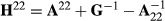 among genotyped animals. Aguilar et al. (2010) and Christensen and Lund (2010) noted that when all genetic variance is not accounted by the SNP effects, the residual polygenic effect can be included into the model using
  instead of G−1 in H22, where Gw = (1-w)G + w A22 and the constant w represent the proportion of polygenic variance not described by markers. In this study, we used w = 0.10. Prior to making Gw, the genomic relationship matrix G was multiplied by scalar
  such that on average diagonals of pedigree and genomic relationship matrices were the same. We build two different genomic relationship matrices, one including information of culled young bull calves (Ginc) and another excluding them (Gexc). The genomic relationship matrices were calculated by method one of VanRaden (2008). Both genomic relationship matrices used the same estimated base population allele frequencies, which were calculated as described by McPeek, Wu, and Ober (2004). Similar to the genomic information, also the pedigree files were built differently: one included the pedigree information of the culled bull calves whilst the other did not. Table 2 shows the numbers of animals in the different pedigrees and H22 matrices.
| Number of animals in pedigree | Number of genotyped animals | |
|---|---|---|
| Excluding culled bulls | 5,173,381 | 21,416 |
| Including culled bulls | 5,182,461 | 30,186 |
Misztal, Vitezica, Legarra, Aguilar, and Swan (2013) noted that when EBV model has unknown parent groups (UPG), they should be taken into account in the ssGBLUP MME as well. So far UPGs have usually included information from the pedigree-based relationship matrix as in the regular animal model. Thus, the groups have ignored genomic information, that is contributions due to  have been ignored in UPG coefficients in MME. Matilainen, Strandén, Aamand, and Mäntysaari (2016) proposed a method to include the impact of the G−1 and
  for the genetic group equations, and this approach was used in our study. In addition, inbreeding coefficients were accounted in computation of A−1 in all models.
The analyses were carried out using the NAV routine evaluation model for EBV milk production (Lidauer et al., 2015). In the evaluations, multiple trait TD model is used to estimate EBVs of milk, fat and protein, simultaneously. Solutions for the MME of the TD model and TD ssGBLUP were computed with MiX99 software using iteration on data and PCG method (Lidauer et al., 2014). Computations for EBVs and GEBVs were very similar; the MME for the TD model to solve EBVs used A−1 which was replaced by alternative H−1 matrices in the ssGBLUP for GEBV. The PCG method was assumed to be converged when Ca was less than 10−6. Statistic Ca is the relative difference between the right-hand and left-hand side of the MME for all the equations describing the additive genetic animal effects (Lidauer et al., 2014). From the TD model solutions, the official 305 days lactation total yield breeding values of milk, protein and fat were derived and used in the analyses (Lidauer et al., 2015).
Study set-up consisted of four different full TD evaluations: two normal TD evaluations using different pedigree information and two ssGBLUP evaluations using different pedigree and genomic information. These are called (G)EBVinc, (G)EBVexc referring to models including or excluding genomic and pedigree information of culled bull calves, respectively. GEBVs and EBVs from the full TD models were compared using Pearson rank correlation coefficients with Fisher's z transformation in SAS (SAS, 2011). Genetic trends and standard deviations (SD) for production traits were obtained by averaging the standardized breeding values of bulls per birth year and comparing the trends obtained from the different TD models.
Validation of the predictions was carried out using Interbull validation protocol (Mäntysaari et al., 2010). For the tests, ssGBLUP and normal TD models were computed using reduced TD data sets. The validation tests were based on 2 or 4 years of data reduction. For the validation of bull GEBVs, the last 4 years of observations were removed from the full data (Rdata4). For the validation of cow GEBVs, only the last 2 years of TD records were excluded (Rdata2). The shorter cut-off period was used for cows, to maintain more female animals with genomic information in reduced data, whilst still having a sufficient number of validation candidates.
From the reduced data analyses, only the bulls that had no daughters in the Rdata4, but had their EBV based on ERC ≥ 3.0 in the full data, were defined as validation bulls. The ERC (effective record contribution) of 3.0 corresponds roughly the phenotypic information obtained from 20 daughters with observations. The ERCs were calculated by the ApaX99 program (Strandèn, Lidauer, Mäntysaari, & Pösö, 2001) for all the animals in pedigree when full data were used. Variance parameters in ERC approximation were from the average daily TD model, and the same values ( = 0.48,
  = 0.48 and
  = 0.49) were used throughout our study. The genotyped cows with no TD records in the Rdata2 and with a minimum of five TD records in the full data were considered as validation cows. Finally, we had 673 validation bulls born between years 2006 and 2009, and 8,572 validation cows born between 2009 and 2012. The ssGBLUP with reduced TD data was run using either with all the genomic data or with excluding the culled bull calves, and the resulting GEBVs were called as GEBVinc,R and GEBVexc,R, respectively.
The EBVs for the weighted three lactation averages were obtained from the full data analysis. These were then deregressed to get deregressed genetic prediction (DRP) for bull and cow GEBV validations. DRPs were obtained using Broyden method in option DeRegress (Strandén & Mäntysaari, 2010) in MiX99 software. The ERC was used as weighting factors in the deregression. The three production traits were deregressed simultaneously but assuming genetic and residual correlations to be zero.

where y is the DRPs of the validation bulls or cows from the full data, and â is the EBVs or the genomic predictions for bulls or cows based on the reduced data analysis. The validation reliability of the model was obtained from the R2 (coefficient of determination) of the model ( ), after correcting it by the average reliability of DRPs
  of the validation bulls or cows, that is
 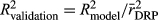 The reliabilities of DRP were calculated as
  where λ = (1 - h2)/h2. To estimate the further gain from the genomic information over the traditional PA (Mäntysaari et al., 2010), the same validation tests were also applied to PA. Confidence intervals (CI) were estimated for the regression coefficients (b1) and the validation reliabilities (R2validation) using non-parametric bootstrap (Koivula, Strandén, Pösö, Aamand, & Mäntysaari, 2015). The boot and boot.ci functions of the R package (Canty & Ripley, 2017) were used to calculate 95% bootstrap CIs. Number of bootstrap samples was 10,000.
3 RESULTS AND DISCUSSION
A number of iterations in solving EBVinc were 4,075, but with ssGBLUP 3,996 and 3,172, for the GEBVinc and for the GEBVexc, respectively. The models took approximately 26 or 58 hr using TD animal model or TD ssGBLUP, respectively, to run with 6 Intel Xeon® 3.6 GHz processors. The iteration time to calculate GEBVinc was approximately 19% longer than for GEBVexc, being 52 and 42 s per iteration round, respectively. Also, the computing time when building genomic relationship matrix was 48% longer when using genomic information including the culled bull calves. The peak virtual memory needed in the construction of the G matrix and inverting it was 13.9 and 7.2 GB for Ginc and Gexc, respectively. For the EBV estimation, there was no difference in iteration time or computational load with different pedigree information. The ssGBLUP in our study was classical computational implementation with full  stored and read from the disc file within each iteration. In practice, the ssGBLUP would likely be implemented using
  (e.g., Fragomeni et al., 2015) or ssGTBLUP (Mäntysaari et al., 2017), making the ssGBLUP more similar to EBV estimation. However, the comparisons of computational demands across different ssGBLUP approaches are justified. It is clear that computational load of TD ssGBLUP can be notably reduced by discarding the genotypes of the culled bull calves from the G matrix.
According to the correlations between EBVs and GEBVs, and their confidence limits (CL), it was apparent that the inclusion or exclusion of the genotypes of the culled bull calves did not affect the (G)EBVs of the reference bulls, common in all TD runs. GEBVs (and EBVs) of the reference bulls were the same whether genomic or pedigree information of the culled bulls was used in the TD model or not (Table 3). For the EBVs, this was as expected, but for the ssGBLUP, it demonstrated that for reliably evaluated bulls, extra information from young genotyped bulls does not change the GEBV estimation. This is partly related to the issue that when a progeny and its sire are both genotyped, the progeny genotype does not provide any additional information to the sire and vice versa (Ducrocq & Liu, 2009). Almost all the test bulls had genotyped sire; 184 of 187 sires were genotyped, and on average, they had 1,736 offspring of which on average 172 were genotyped sons. However, nearly all of the reference bulls were chosen for AI before the era of genomic selection, so the near-unity correlation for these bulls might not imply unity correlation for genomically selected bulls after they have progeny. The genetic trends or the SDs in the reference bulls did not change even when genomic information of culled bulls was used. Figure 1 shows the genetic trends and Figure 2 the SD for protein (G)EBVs. Only one EBV trend is presented in the figures because the EBV trends by including or excluding the culled bulls were exactly the same.
| Reference bulls | Test bulls | |||
|---|---|---|---|---|
| Correlation | 95% CL | Correlation | 95% CL | |
| EBVinc* EBVexc | 1.00 | 1.00–1.00 | 1.00 | 1.00–1.00 |
| GEBVinc* GEBVexc | 0.99 | 0.99–0.99 | 0.97 | 0.96–0.97 |


Our study indicated that including genomic information of the culled bull calves without progeny has some effect on the genomic evaluation of the test bulls to be progeny tested. The correlation between GEBVinc and GEBVexc was 0.97 for the test bulls group (Table 3), and in the most cases, GEBVinc was higher than GEBVexc (Figure 3). In general, the GEBVs of the test bulls had a tendency to have higher GEBVs compared to their EBVs (or PAs in the case of test bulls). The difference was even higher when genomic information of the culled bull calves was included in the ssGBLUP evaluation. This can be observed also in the genetic trend for protein which was estimated higher for the test bulls when the culled bulls had been included in ssGBLUP evaluation (Figure 1). Similar trends were observed also for milk and fat yields, although only a protein yield trends are presented. When we checked the GEBV trends and mean level for the culled bull calves (results not shown here), these were found to be clearly lower than those of the test bulls. Thus, there is a tendency that GEBVs of the test bulls get higher if genotypes of their culled half-sibs are included in the ssGBLUP evaluation. As expected, the SD of GEBVs for the test bulls within birth years was higher than those of the PA due to the extra information from the genotypes (Figure 2). However, the inclusion of genomic information for the culled bull calves did not have a clear effect on the SD of GEBVs, although there was a tendency that SD is higher if culled bulls are included in the ssGBLUP.

An important question is whether the (G)EBVs of the bull sires and bull dams change when information of their culled offspring is included in the model or not. As expected, EBVs of parents to the test bulls did not change when culled bulls were included in the pedigree because the culled bull calves had no observations nor progeny. Thus, the correlation between EBVs for these parents was one. Correlation between GEBVinc and GEBVexc for the test bull parents was 0.99. Therefore, it appeared that also GEBVs of the bull sires and dams are more or less the same whether or not genotypes of their culled sons are used in the ssGBLUP evaluation.
The model validation results for the bulls are in Table 4 and for the cows in Table 5. Tables present regression coefficients (b1) and validation reliabilities (R2) with 95% bootstrap confidence intervals (CI). For the bulls, validation reliabilities from the ssGBLUP were 0.43 and 0.44 for milk, 0.34 and 0.34 for protein and 0.37 and 0.38 for fat, when genotypes of the culled bull calves were included (GEBVinc,R) and excluded (GEBVexc,R), respectively (Table 4A). The PA based on the same data but without genomic information gave on average 9.6% units lower reliability for all traits. These numbers are lower than those we have obtained in our earlier studies (Koivula et al., 2015), where the R2 has been on average 0.49 for milk, 0.40 for protein and 0.44 for fat. The reason for decreased validation reliabilities may be partly in the different genomic matrix (e.g., use of base population allele frequencies or accounting phantom parent groups in the G matrix), but may also be related to the preselection of genotyped young animals in the current study. For the cows, validation reliabilities with different genomic data were 0.34 and 0.38 for milk, 0.28 and 0.31 for protein and 0.29 and 0.31 for fat, when genotypes of the culled bulls were included (GEBVinc,R) and excluded (GEBVexc,R) respectively. Cow PA gave on average 5.6% units lower reliabilities than GEBVs. However, for the cows, the validation reliabilities can differ also because they have less close relatives in the reference population. The inclusion of genotypes of the culled bull calves did not have a large effect on validation reliability of validation bulls or cows. However, there was a slight tendency that R2 was lower when genomic data of the culled bulls were included in the ssGBLUP evaluation. In general, differences in the validation reliabilities were quite small between the ssGBLUP evaluations that included or excluded genotypes of the culled bulls. This is demonstrated by 95% bootstrap confidence intervals (CI) that indicate that main differences appear between PA and different GEBVs.
| Method | Milk | Protein | Fat | |||
|---|---|---|---|---|---|---|
| b1 | R 2 | b1 | R 2 | b1 | R 2 | |
| (A) | ||||||
| PA | 0.95 (0.84–1.06) | 0.36 (0.29–0.42) | 0.80 (0.69–0.92) | 0.26 (0.19–0.33) | 0.68 (0.59–0.78) | 0.24 (0.18–0.30) |
| GEBVinc,R | 0.74 (0.67–0.81) | 0.43 (0.37–0.50) | 0.60 (0.53–0.68) | 0.34 (0.27–0.41) | 0.65 (0.58–0.72) | 0.37 (0.31–0.43) |
| GEBVexc,R | 0.76 (0.69–0.83) | 0.44 (0.37–0.50) | 0.63 (0.56–0.71) | 0.34 (0.28–0.41) | 0.67 (0.60–0.74) | 0.38 (0.31–0.44) |
| (B) | ||||||
| PA | 0.71 (0.55 – 0.87) | 0.27 (0.15–0.37) | 0.65 (0.48–0.84) | 0.24 (0.11–0.35) | 0.75 (0.57–0.91) | 0.29 (0.18–0.39) |
| GEBVinc,R | 0.72 (0.63–0.84) | 0.44 (0.33–0.55) | 0.64 (0.55–0.78) | 0.39 (0.26–0.52) | 0.73 (0.65–0.86) | 0.46 (0.36–0.57) |
| GEBVexc,R | 0.74 (0.64–0.84) | 0.44 (0.33–0.55) | 0.66 (0.55–0.78) | 0.39 (0.26–0.52) | 0.76 (0.65–0.86) | 0.47 (0.36–0.57) |
| Method | Milk | Protein | Fat | |||
|---|---|---|---|---|---|---|
| b1 | R 2 | b1 | R 2 | b1 | R 2 | |
| PA | 0.96 (0.91–1.02) | 0.30 (0.26–0.32) | 0.89 (0.84–0.95) | 0.26 (0.22–0.28) | 0.84 (0.78–0.89) | 0.23 (0.20–0.25) |
| GEBVinc,R | 0.65 (0.61–0.69) | 0.35 (0.34–0.41) | 0.55 (0.52–0.58) | 0.28 (0.24–0.31) | 0.59 (0.55–0.62) | 0.30 (0.26–0.32) |
| GEBVexc,R | 0.75 (0.71–0.78) | 0.38 (0.34–0.41) | 0.64 (0.60–0.68) | 0.30 (0.26–0.33) | 0.67 (0.63–0.71) | 0.32 (0.28–0.34) |
The degree of inflation is indicated by the coefficient of regression (b1) of true genetic values on (G)EBV. Optimal prediction of genetic merit of young individuals should have a regression coefficient of one. With b1 less than one, the predictions are inflated, and the differences in estimated genetic merit of the test individuals are biased upwards compared to their future performance. For the validation bulls, the b1 coefficients were always lower than the expected value, indicating that GEBV exaggerated differences between bulls (Table 4). Moreover, b1 coefficients were even lower with the ssGBLUP evaluation that included genomic information of the culled bulls. A similar trend was observed also in the cow validation (Table 5). The bull validations were also conducted with 2 years of data reduction (like in cows). With this validation, we had 256 validation bulls, and the validation reliabilities from the ssGBLUP were higher compared to the validation with 4 years of data (Table 4B). Thus, it was clear that more genotyped cows in the reference population improved the validation of bulls. Still, the difference between the two ssGBLUP evaluations remained: the b1 values were a bit higher with GEBVexc,R than with GEBVinc,R.
Validation results (both b1 and R2 values) indicated that inclusion of genotypes of the culled bull calves may increase bias in the ssGBLUP evaluation. This was more evident in the cow validation. Therefore, it might be reasonable to discard the genomic information of culled bull calves. This could decrease overestimation of GEBVs of test bulls and improve validation reliability of bulls and cows. This will also reduce computational load of the TD ssGBLUP evaluation. The inclusion of all genomic data in ssGBLUP evaluation is a reasonable principle because in theory, all information used in making selection decisions should be accounted in the genetic evaluation. Ducrocq and Liu (2009), and Patry and Ducrocq (2011) underline the importance of all animals in the genetic evaluation, and Shabalina et al. (2017) reported that information from culled animals improved accuracy of the ssGBLUP. One argument to taking all information in the genomic evaluations is that in that way we can take better into account genomic preselection. However, in genomic preselection, the bull calves are culled based on their GEBV and therefore do not provide any phenotypic information about selection. Moreover, based on the current results, the culled bulls in ssGBLUP might not need to be included in the single-step evaluations.
In the ssGBLUP evaluations, it is important to make the pedigree (A) and genomic (G) matrices compatible (e.g., Meuwissen, Luan, & Woolliams, 2011). We ensured compatibility using inbreeding coefficients in A−1, base population allele frequencies in G and blending of a properly scaled G matrix with pedigree matrix A22. An approach that can diminish bias in the evaluation is use of weights on G−1 and  , that is
  (Tsuruta, Misztal, Aguilar, & Lawlor, 2011). We tested a case with τ = 1 and ω = 0.7 for our set-up in this study. Use of these parameters decreased bias but still the evaluations would have failed the Interbull requirement of having the variance inflation coefficient b1 equal to one.
4 CONCLUSIONS
Both the full and the reduced TD data models indicated that inclusion of genomic information of culled bull calves without progeny may increase bias in the ssGBLUP evaluation. When full TD data were used, the GEBV trend of young test bulls, which were bought for AI, was higher if genotypes of the culled bull calves were included in the ssGBLUP evaluation. In the validation test, there was a tendency that validation R2 and b1 coefficient were better if genotypes of the culled bulls were excluded from the ssGBLUP evaluation.
ACKNOWLEDGEMENTS
This work was a part of the Genomic in Herds project originally established by Luke, Aarhus University and Nordic Cattle Genetic Evaluation Ltd (NAV, Aarhus, Denmark). Viking Genetics (Randers, Denmark), Faba (Hollola, Finland), Valio (Helsinki, Finland) and MAKERA foundation (Finnish Ministry of Agriculture and Forestry) are acknowledged for financial support.