Mortality Portfolio Risk Management
ABSTRACT
We provide a new method, the “MV+CVaR approach,” for managing unexpected mortality changes underlying annuities and life insurance. The MV+CVaR approach optimizes the mean–variance trade-off of an insurer's mortality portfolio, subject to constraints on downside risk. We apply the method of moments and the maximum entropy method to analyze the efficiency of MV+CVaR mortality portfolios relative to traditional Markowitz mean–variance portfolios. Our numerical examples illustrate the superiority of the MV+CVaR approach in mortality risk management and shed new light on natural hedging effects of annuities and life insurance.
INTRODUCTION
Life insurance companies sell a wide variety of life insurance and annuity products. The insurers' liabilities for these products depend on future mortality rates. During recent years, economic and demographic changes have made mortality projection and risk management more important than ever. On the one hand, life expectancy for ages 60 and older in the past two decades has improved at a much higher rate than what pension plans and annuity providers expected. Cowling and Dales (2008) find that companies in the United Kingdom FTSE100 index underestimated their aggregate pension liabilities by more than £40 billion. If the firms do not take measures to control mortality downside risk, such longevity shocks are likely to cause serious financial consequences. For example, unanticipated mortality improvement was an important factor accounting for the failure of Equitable Life, once a highly regarded U.K. life insurer (Ombudsman, 2008). On the other hand, population growth, urbanization, and increased global mobility may lead to a more rapid and widespread disease. Genetic analysts recently confirmed that today's “bird flu” is similar to the 1918 “Spanish flu” that killed more than 40 million people. This finding spurs fears of a worldwide epidemic (Juckett, 2006). According to Toole (2007), losses due to a severe pandemic could amount to 25 percent of the U.S. life insurance industry's statutory capital. While the great majority of U.S. life insurance companies would weather such a pandemic, it is clear that these companies should be interested in mitigating the risk.
We propose a method that life insurance companies can use to alleviate extreme mortality outcomes while maintaining a relatively efficient mean–variance relationship for their mortality portfolios of life insurance and/or annuities. This method, the “MV+CVaR approach,” combines Markowitz mean–variance (MV) portfolio theory and conditional value at risk (CVaR) by optimizing the trade-off between mean and variance subject to an upper bound on CVaR. Variance measures both positive and negative deviations of portfolio values from its expected level, while CVaR focuses on the portfolio tail loss caused by extreme events. Although the MV+CVaR portfolios are suboptimal relative to the Markowitz counterparts in terms of the mean–variance efficiency, they are attractive to insurers since the MV+CVaR portfolios have lower downside risk while achieving desirable risk–return trade-offs. In practice, life insurers are keenly interested in searching for an optimal risk–return relationship for their business. At the same time they are required to meet various solvency requirements for possible catastrophes such as flu epidemics. Therefore, incorporating both variance and CVaR as risk measures in business optimization such as the MV+CVaR approach should be appealing to life insurance companies. The risk control framework adopted in this article closely follows that of Rockafellar and Uryasev (2000) and Tsai, Wang, and Tzeng (2010). In their framework, firms minimize portfolio losses subject to CVaR constraints. In our context, we consider both variance and CVaR as risk measures by incorporating a CVaR constraint into the classical mean–variance setup.
We extend Rockafellar and Uryasev (2000) and Tsai, Wang, and Tzeng (2010) in one important dimension by applying the well-developed moments method to validate the quality of MV+CVaR portfolios. The existing literature on mortality models usually makes distributional assumptions. Since knowledge about the underlying mortality distributions may be limited, the assumed distributions may not represent the actual mortality dynamics. However, the moments method is solely based on moments, not a specific distribution. This method yields robust semiparametric upper and lower bounds that any reasonable model with the same moments must satisfy. Once a mortality portfolio has been constructed, the corresponding empirical benefit payments can be used to estimate moments of the benefit payment ratios. In this article, we show how such estimated moment information can be used to determine the bounds on the underlying portfolio benefit payment ratios. In particular, the moments method provides a mechanism to compare the downside risk of a MV+CVaR efficient mortality portfolio and its MV counterpart given their moments. Our results show the superiority of the MV+CVaR approach in mortality risk management and highlight the natural hedging effects of life insurance and annuities.
For the numerical examples, all optimization problems are solved with matlab1 software. When computing the bounds of a particular portfolio, we solve the equivalent dual problem using built-in functions from the SOS programming solver. The SOS programming solver was developed by Prajna et al. (2004), which is a free toolbox written in MATLAB. Our implementation is fairly general and easy to use.
The remainder of this article is organized as follows. The first section describes how to calculate benefit payment ratios of mortality portfolios. The second section discusses the MV+CVaR mortality optimization model. We provide two numerical examples to illustrate the implementation of the approach. The third section describes the method of moments. We show how to compute the semiparametric upper and lower bounds for MV+CVaR efficient portfolios and then perform the bound analysis on those portfolios. The fourth section demonstrates the natural hedging effect when annuities and life insurance are considered jointly. The fifth section extends the analysis to efficient frontiers of MV+CVaR mortality portfolios by comparing bounds of MV and MV+CVaR optimal portfolios. In addition, we show to what extent downside risk is reduced by changing the CVaR constraint. The sixth section is our conclusion.
MORTALITY RISK PORTFOLIOS
Focus on Mortality
- All future cash flows are discounted at risk-free interest rates. These discount rates are known constants.
- Life insurance policies and annuity contracts remain in force until settled at death. There are no policy lapses.
- Expenses are known constant multiples of policy premiums.
- The analysis is applied only to new business without regard to the insurer's book of business issued before time 0.
Under these assumptions, the present value of benefits (and related expenses) paid at times 1, 2, … , PVB (x), and the present value of premiums (and related expenses) collected at 0, 1, 2, … , PVP (x), are simple functions of the lifetime K(x). The randomness of the present values has two components. First, future mortality events will have an impact on annual survival rates for members of the class (x). That is, the annual survival rate p(x)+ t for the year running from t to t+1 is random for t=1, 2, … . Given a random path of the survival rates  , we can calculate the conditional distribution of the lifetime K(x). But some randomness still remains. However, the remaining randomness is subject to the law of large numbers; if the company writes a large enough number of policies in each underwriting class, it can be ignored. Therefore, we focus on the conditional expected values
  and
and  .
.
We assume the company uses the benefit payment ratio  to manage its risk where
  is a constant expense ratio. Other measures are possible; for example, one might use
  . The benefit payment ratio is analogous to the loss ratio used in general (non-life) insurance where policies are much more often single premium (and single period) contracts.
The benefit payment ratio is a random variable as viewed from time 0, but only due to the uncertainty of future mortality rates. We give some examples below to illustrate the calculation of the benefit payment ratio. The company has a model for generating paths  , and from them it generates a sample of values of
  . Moments of these sample distributions are inputs to the mortality risk management process. In our examples, we will use the Lee–Carter model (Lee and Carter, 1992) to generate future paths of the survival rates p(x)+ t, or equivalently the death rates q(x)+ t =1− p(x)+ t. In principle there are many methods that could be used; the company may have its own proprietary method.
In practice the insurance company will consider more than one line of business at 0; let (xi) denote a set of underwriting classes under consideration at 0. For example, (x1) might be male, 10-year term life insurance issued at age x1 =35; (x2) might be an immediate annuity issued to a female age x2 =65; and so on. The company jointly simulates paths for each class. This is much more difficult than simulating a single path. The Lee–Carter method has been extended to handle this situation (Li and Lee, 2005). Brouhns, Denuit, and Vermunt (2002) show how an extension of the Lee–Carter model can be used to jointly model annuitants and the general population to which they belong. Hyndman, Booth, and Yasmeen (2011) describe another generalization of Lee–Carter that allows for joint modeling of components of a population. However, these methods are still being developed. Moreover, there is very little publicly available data on insured lives and annuitants. Therefore, we will use a single mortality table forecast. There are circumstances where it is appropriate. For example, if we consider 10-year term insurance issued at 0 to a male age (35) and 20-year term insurance issued at 0 to a male age (45), then it is reasonable to use mortality rates from the same table that differs only by age. That is, we need to project only one table and then select values from it for the appropriate ages.
Examples
 is the ratio, calculated at 0, of the conditional expected present value of benefits to the conditional expected present value of future premiums for the contract issued on (x), with the conditional distribution of K(x) calculated relative to a given future path of the underlying mortality table. For example, given a path of future survival rates
  for (x), we can calculate the conditional survival function of K(x) as
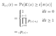 (1)
(1) (2)
(2)Life Insurance
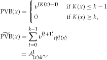 (3)
(3) is the same as the present value of benefits for a whole life insurance; in this case A(x) is analogous to the standard actuarial notation.
 per unit of benefit at that time, then the benefit payment ratio is simply
  where the conditional expected value of premiums
  equals
 (4)
(4)Immediate Annuity
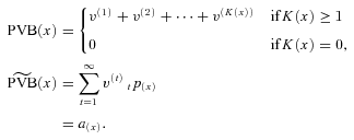 (5)
(5) where P is the single premium paid at 0 per unit of annual benefit.
In the next section we consider an insurer selling several lines of business at time 0 and optimize its portfolio. In order to do this we need statistical samples of the benefit payment ratios of lines of business under consideration, which we obtain by Monte Carlo simulation.
MORTALITY PORTFOLIO OPTIMIZATION
The original Markowitz portfolio optimization (Markowitz, 1952) maximizes an investor's expected portfolio return for a given level of risk, as measured by the variance of the return. More recent portfolio optimization techniques have been applied to corporate risk management to find optimal business strategies. For example, insurers are motivated to search for business compositions that not only achieve mean–variance efficiency but also minimize downside risk. In this section, we extend this line of research by adding capital constraints to the Markowitz problem for managing an insurer's mortality portfolio.
Portfolio Optimization With CVaR Constraints
The conditional value at risk (CVaR) is a risk measure, defined as the expected loss conditional on the benefit payment ratio being higher than a given value at risk (VaR). The existing literature has many CVaR-related portfolio management methodologies. For example, Rockafellar and Uryasev (2000) generate an efficient  -mean frontier by minimizing the CVaR of portfolio's losses subject to an expected return requirement. Krokhmal, Palmquist, and Uryasev (2002) suggest minimizing the negative expected return with a CVaR constraint. In the context of mortality risk management, we explicitly consider the trade-off between mean and variance subject to CVaR constraints by adding a CVaR constraint to the traditional Markowitz problem. We call it the MV+CVaR approach.
 . Let
. Let  denote the covariance of benefit payment ratios of business lines i and j. Our MV+CVaR problem is to solve for portfolio weights
  in terms of benefit payment ratios, so as to
 (6)
(6) is the
  -level CVaR of
  , which in the case of a continuously distributed
  can be calculated as

 -level value at risk,
  , is the
  -quantile of the distribution of
  , or the smallest value of
  such that
  . That is,

 at 0.95. The CVaR constraint in (6) ensures the tail expectation
  is no higher than a prespecified value
  , thus reducing the downside risk.
  is a subset of the mortality business feasible set. Specifically in our problem,
  is the vector of weights
  satisfying
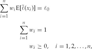 (7)
(7) is the random benefit payment ratio of line i, n is the number of business lines in the mortality portfolio, and
  is a prespecified level of the weighted average of the benefit payment ratios. We assume that
  for each i. Negative values would indicate the insurer buys insurance rather than selling. It is possible to do this in practice with reinsurance, but we are not allowing it in our model.
 -level CVaR is the optimal value of the following optimization problem
 (8)
(8)
 (9)
(9) achieves the minimization of (9),
  will return a
  -level CVaR and
  will give the corresponding
  -level VaR. For the detailed proof of the theorem, see Theorem 4 of Krokhmal, Palmquist, and Uryasev (2002).
Here, we present the equivalence of the CVaR constraint (i.e.,  ) and the constraint
  in the form shown in (9) that will be suitable for our purpose, instead of presenting it in its general form proposed by Krokhmal, Palmquist, and Uryasev (2002). In general, if the objective function is convex and the constraints (other than the CVaR constraint) are linear, one can replace the CVaR constraint in the optimization problem with
  .
.
 has a tractable formulation. Using a well-known linearization technique, adding auxiliary variables yk for
  , the constraint
  can be realized as
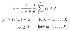 (10)
(10) is calculated as the mean of K equiprobable observations,

Numerical Illustration
Now we conduct numerical experiments for a life insurer's business portfolio to illustrate the superiority of the MV+CVaR approach to the MV approach. Example 1 demonstrates the case of an insurance company considering three lines of business. Example 2 extends the analysis to a larger scale problem of an insurer considering nine business lines.
Example 1
- The annual level premiums
 are the average market prices in 2005 for i=1, 2, 3.
 - The insurer uses the Lee and Carter (1992) model to simulate 150 future mortality paths. Because we do not have a time series of insured life tables, we use population data. An insurer would very likely use its own data.
- The insurer uses the U.S. Treasury yield curve on December 28, 2005 to compute the benefit payment ratios based on Formula (3).
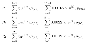 (11)
(11) for each line of business. This means expenses are 12.5 percent of premiums, paid at the same time as the premiums are collected. Therefore, the benefit payment ratios by line in year 0 are
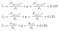 (12)
(12) in place of
  . We simulated a future path of mortality, for that path calculated the values of
  ,
,  , and A(40) using (3) and those of P1, P2, and P3 using (11), and then calculated the benefit payment ratios using (12). One path of mortality yields one joint observation of the three benefit payment ratios. We repeat this 150 times. The Appendix shows some details on the Lee and Carter (1992) method we used to simulate those tables.
Table 1 shows the descriptive statistics for the benefit payment ratio of these three lines of life insurance based on 150 trials of simulation. It turns out that the 10-year term life insurance (i=1) on a male age (25) has the lowest mean benefit payment ratio and the highest variance. The whole life insurance (i=3) on a male age (40) has a higher mean benefit payment ratio and lower variance than the 5-year term life insurance (i=2) on a male age (35).
| Line | Mean | Variance | Skewness | Kurtosis | ||
|---|---|---|---|---|---|---|
| i | Age | Type | ||||
| 1 | (25) | 10-year term | 0.8587 | 0.0083 | 0.3576 | 0.2481 |
| 2 | (35) | 5-year term | 0.9403 | 0.0055 | 0.2997 | 0.6804 |
| 3 | (40) | Whole life | 0.9710 | 0.0045 | 0.3631 | 0.1024 |
 (13)
(13) are shown in the row labeled “Original” in Table 2 for the same 150 simulations that we used in Table 1. To search for an optimum business strategy, we solve the MV+CVaR optimization Problem (9). We specify

 (14)
(14) is the 95 percent level CVaR of the original portfolio. The specification (14) controls the downside risk by reducing the original 95 percent level CVaR by
  . The firm can set a different risk reduction level to fit its particular situation. Later we will show how an adjustment in risk reduction level
  changes the optimal solution. With (14) we get the following weights for the MV+CVaR optimal business composition:

 |
Mean | Variance | Skewness | Kurtosis | Mode | CVaR 95% |
|---|---|---|---|---|---|---|
| Original | 0.9567 | 0.0043 | 0.2912 | −0.0182 | 0.9591 | 1.1047 |
| MV+CVaR | 0.9567 | 0.0038 | 0.1457 | −0.2772 | 0.9755 | 1.0802 |
Example 2
Now we include more life insurance lines and analyze a larger scale problem with nine lines of life insurance: 5-year term, 10-year term, and whole life insurance issued at ages (25), (35), and (40). The sample statistics of these nine lines are summarized in Table 3. These sample statistics come from a different set of simulations from that in 1, so the sample statistics are not exactly the same as those in Table 1 but they are very close and qualitatively the same.
| Line | Mean | Variance | Skewness | Kurtosis | ||
|---|---|---|---|---|---|---|
| i | Age | Type | ||||
| 1 | (25) | 5-year term | 0.8369 | 0.0044 | 0.1810 | −0.1170 |
| 2 | (35) | 5-year term | 0.9346 | 0.0054 | 0.1444 | −0.1219 |
| 3 | (40) | 5-year term | 1.1238 | 0.0060 | 0.1032 | −0.1131 |
| 4 | (25) | 10-year term | 0.8534 | 0.0073 | 0.0500 | −0.1606 |
| 5 | (35) | 10-year term | 1.2023 | 0.0131 | −0.0274 | −0.0724 |
| 6 | (40) | 10-year term | 1.4035 | 0.0128 | −0.0888 | −0.0200 |
| 7 | (25) | Whole life | 0.7274 | 0.0068 | 0.0497 | −0.0961 |
| 8 | (35) | Whole life | 0.8842 | 0.0054 | −0.0873 | −0.2010 |
| 9 | (40) | Whole life | 0.9632 | 0.0045 | −0.1202 | −0.2478 |
We assume the insurer originally has equal weights on each line of business (i.e.,  . Given this assumption, the summary statistics of this evenly weighted portfolio are shown in the row labeled “Original” in Table 4. The expected benefit payment ratio of the original nine-line portfolio is 0.9921 and its variance is 0.0055.
 |
Mean | Variance | Skewness | Kurtosis | Mode |  |
|---|---|---|---|---|---|---|
| Original | 0.9921 | 0.0055 | −0.1264 | −0.3395 | 0.9382 | 1.1301 |
| MV+CVaR | 0.9921 | 0.0036 | −0.1950 | −0.5096 | 0.9941 | 1.0960 |

 determined by Equation (14). The MV+CVaR optimal business composition solution is

BOUNDS ANALYSIS WITH THE METHOD OF MOMENTS AND MAXIMUM ENTROPY
How well does the optimal business strategy secure an insurer's financial position? In this section, we apply the method of moments to address this problem. In addition, we allow for higher order moment information to be included in the mortality risk management setup.
Here is the setting of a reasonably general moment problem. Given moments  and an interval [b1, b2 ], let
  denote the set of random variables Z with support in [b1, b2 ] (i.e.,
  with probability 1) and
  for
for  . Let
. Let  be a well-behaved real-valued function defined on [b1, b2 ]. The moment problem is to determine the best upper and lower bounds on
  , over all random variables
  , given
  for
for  . These ideas have roots in the work of Tchebyshev, Markov, and Stieltjes in the 1870s. Tian (2008) provides a detailed discussion of moment problems in portfolio risk management.
 for
for  and
and  for z > d, so that
  is the survival function of Z. The solution to the moment problem below produces bounds on
  :
:
 (15)
(15) satisfying
  for
for  . Similarly, the problem for the lower bound of
  is the solution of the following problem:
 (16)
(16)In our analysis, we are interested in the bounds on the survival function of the weighted average benefit payment ratios, that is,  , where
  is the weighted average benefit payment ratio of a mortality portfolio, defined previously.
This moment problem can be solved numerically with semidefinite programming solvers such as SOSTOOLS (Prajna et al., 2004). See Akhiezer (1965), Parrillo (2000), Popescu (2005), and Bertsimas and Popescu (2005) for the details on applying semidefinite programming solvers to the bound Problems (15) and (16).
Unimodal Bounds
Adding a distribution assumption such as unimodal to the constraints in (15) or (16) means that we optimize over a smaller set and thus obtain tighter bounds than the general bounds. Since many data sets have unimodal empirical distributions, we find the unimodal assumption appealing. However, one has to be aware that the resulting bounds are valid only if the variable (benefit payment ratio in our case) has a unimodal distribution. If the distribution is not unimodal, then implementing moment analysis with a unimodal assumption may eliminate important tail behavior.
 is replaced by

 . And the bounds
  are replaced by
  where
where

 and
and  . The general bounds on the survival function of
  always satisfy
 (17)
(17) has a unimodal distribution the following relationship applies
 (18)
(18) and
and  ) with their unimodal counterparts, we have
  .
.Maximum-Entropy Distribution
The work of Shannon (1948a,1948b) in information theory and Jaynes (1957) in statistical physics led eventually to the concept of entropy in probability theory. The entropy of a probability distribution is a measure of how much information it contains. The maximum-entropy distribution is the “most likely,” “most unbiased,” “least prejudiced,” or “most uniform” distribution of a given class of distributions.
 of distributions on [b1, b2 ] with given moments
  for
for  ; these are the distribution functions of the random variables Z in
  give in the previous section. The entropy of a continuous type distribution
  is defined as

 with maximum entropy is the solution to the following moment problem
 (19)
(19) (20)
(20) are Lagrange multipliers associated with the constraints defining
  and
and

 is the distribution using as little information as possible (using only moments) to analyze the risk of MV+CVaR mortality portfolios.
Numerical Illustrations
Now we apply the bound and maximum entropy analysis to the numerical examples in the previous section.
Example 1
 (21)
(21) (22)
(22) curves. The normal distribution (the dotted lines in Figure 2) with the same mean and variance as the original mortality portfolio must fall between the two-moment upper and lower unimodal bounds. In this example, the normal curve is even within the four-moment unimodal bounds. Under the normal assumption, the business's VaR 95percent is 1.065.
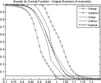
Bounds of the Original 3-Line Life Insurance Portfolio
Notes: The lines with  are the upper and lower general bounds of (17) with four moments. The solid lines show the unimodal bounds of (18) with four moments and the unimode 0.9591. The dotted line in the middle represents the normal distribution with the same mean and variance as the original 3-line portfolio. The vertical axis stands for the survival probability
  , and the horizontal axis represents d (for this and similar graphs that follow).
 (23)
(23)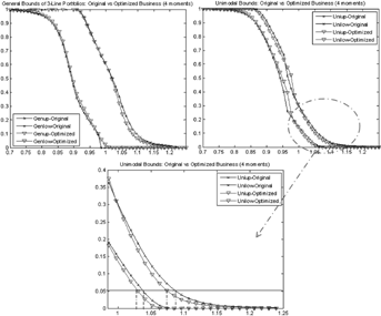
Notes: The upper left plot shows the general bounds. The unimodal bounds are shown in the upper right plot. The plot in the bottom is an enlargement of the unimodal bounds. In all plots, the lines with  represent the upper and lower bounds of the original business. Bounds on the optimal MV+CVaR business strategy are shown in the
  curves.
To take our discussion one step further, we solve the maximum-entropy Problem (19). The results are shown in Figure 4, which compares the maximum-entropy distributions of the original and the MV+CVaR mortality portfolios. In particular, the right tail of the MV+CVaR three-line portfolio shifts to the left of the original portfolio distribution. Therefore, the optimized portfolio has lower downside risk than the original one, which is consistent with the conclusion of the bound analysis.
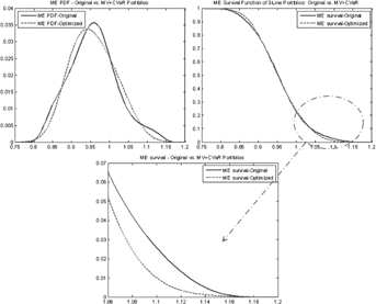
Notes: The upper left plot graphs the density functions  and the upper right one shows the survival function
  . The third plot in the bottom is an enlargement of the survival function shown in the upper right plot. The solid curves are for the original portfolio and the dash lines are for the MV+CVaR optimum.
Example 2
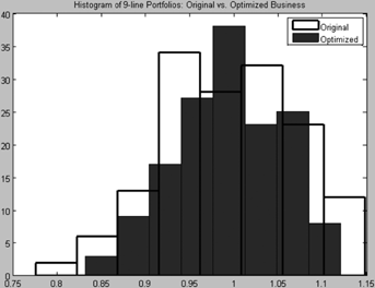
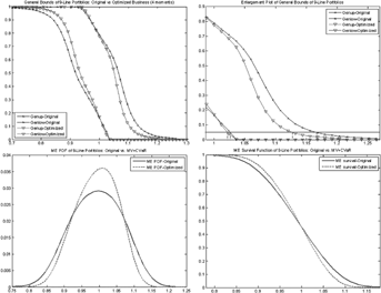
Continuing with Example 2, Figure 5 shows the histograms of the nine-line original and MV+CVaR optimal portfolios with eight bins. Since neither portfolio distribution is unimodal, we only compute their four-moment general bounds. Figure 6 illustrates their four-moment general bounds and maximum-entropy survival functions. Again the right tail of the MV+CVaR optimal portfolio lies on the left of that of the original portfolio in the bound and maximum-entropy analyses, implying lower shortfall risk after optimization.
NATURAL HEDGING EFFECTS
Cox and Lin (2007) argue that an insurer selling both life insurance and annuities is exposed to lower one-directional changes in mortality. This effect is called “natural hedging.” That is, adding annuities to a life insurance portfolio may lower the portfolio's mortality risk. In this section, we examine how natural hedging improves the MV+CVaR optimal business composition and decreases downside risk with the method of moments.
Example 1
To illustrate the natural hedging effect, we add an annuity to the three-line life insurance portfolio analyzed in Example 1. Specifically, in addition to selling the three life policies, the insurer also sells a single premium immediate life annuity on male age (65). Assume that the insurer sells the annuity at the average market quote of 2005, which charges a monthly payout rate of $6.56 per lump-sum premium $1,000 (Stern, 2008). We further assume that the insurer uses the same mortality data and method as those for life insurance to forecast the future survival payments of annuities.
As we mentioned earlier, we are using a single times series of mortality, the U.S. male population data, as the basis for the mortality forecasts. The summary statistics for the benefit payment ratio of this annuity,  , with an expense ratio of
  , are shown in Table 5.
| Line | Mean | Variance | Skewness | Kurtosis | ||
|---|---|---|---|---|---|---|
| i | Age | Type | ||||
| 10 | (65) | Immediate annuity | 0.9924 | 0.0002 | −0.1071 | −0.0074 |

 at 0.9652, same as the expected benefit payment ratio of the original portfolio, and construct a 95 percent CVaR constraint with
  in (6) determined by Equation (14). We get the MV+CVaR efficient four-line mortality portfolio with the weights,
 (24)
(24) |
Mean | Variance | Skewness | Kurtosis | Mode | CVaR 95percent |
|---|---|---|---|---|---|---|
| Original | 0.9652 | 0.0011 | 0.2671 | −0.1178 | 0.9636 | 1.0383 |
| MV+CVaR | 0.9652 | 9.11E-05 | 0.7142 | 1.0956 | 0.9608 | 0.9886 |
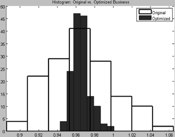
Figure 8 shows the four-moment unimodal bounds and the maximum-entropy distributions of the original and MV+CVaR portfolios with four lines of business. The probability density function of the MV+CVaR optimal four-line portfolio is much tighter than that of the original portfolio, so the upper and lower unimodal bounds of the MV+CVaR portfolio are narrower.
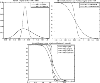
Notes: The upper left plot shows the maximum-entropy probability densities. The upper right plot shows the corresponding survival functions. In both graphs, the solid curves represent the original portfolio and the dash lines draw the MV+CVaR optimum. The plot at the bottom draws the unimodal bounds. In the bottom plot, the curves with  stands for the bounds of the original portfolio and the bounds of the optimized one are represented by the
  curves.
To explore the natural hedging effect, we compare the bounds of the MV+CVaR three-line and four-line portfolios. If we assume both the optimized portfolios have unimodal distributions, the right plot in Figure 9 shows how the 100 percent confidence interval of the 95 percent level VaR improves by adding an annuity to the three-line pure life insurance portfolio. The confidence interval of VaR 95percent of the four-line portfolio stays at a much lower level of benefit payment ratio range than that of VaR 95percent of the three-line portfolio. It highlights the benefits of natural hedging: by including both annuity and life insurance in a portfolio, natural hedging reduces benefit payment and decreases mortality risk.
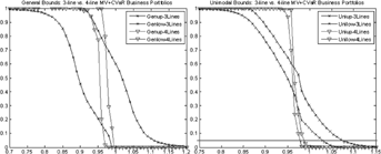
Notes: The left graph shows the general bounds and the unimodal bounds are shown on the right. In both plots, the curves with  represent the upper and lower bounds of the MV+CVaR portfolio with three lines of life insurance. Bounds on the optimal 4-Line mortality portfolio are shown as the
  curves.
Example 2
We add three immediate annuities on male with issue ages (65), (70), and (75) to the nine-line life insurance portfolio we discussed in previously. The sample statistics of these three annuities are given in Table 7. The sample statistics of the immediate life annuity on male age (65) come from a different set of simulations from Example 1. So its moments are not exactly the same as those in Table 5 but they are very close and qualitatively the same.
| Line | Mean | Variance | Skewness | Kurtosis | ||
|---|---|---|---|---|---|---|
| i | Age | Type | ||||
| 10 | (65) | Immediate annuity | 0.9938 | 0.0002 | 0.3246 | −0.0847 |
| 11 | (70) | Immediate annuity | 0.9801 | 0.0003 | 0.3797 | 0.0553 |
| 12 | (75) | Immediate annuity | 0.9707 | 0.0003 | 0.4179 | 0.2097 |
 ). By adding 95 percent CVaR constraint to the Markowitz problem and specifying the expected benefit payment ratio

 (25)
(25) |
Mean | Variance | Skewness | Kurtosis | Mode | CVaR 95percent |
|---|---|---|---|---|---|---|
| Original | 0.9895 | 0.0027 | −0.1069 | −0.3555 | 0.9521 | 1.0865 |
| MV+CVaR | 0.9895 | 3.89E-06 | 0.5264 | 0.8525 | 0.9880 | 0.9940 |
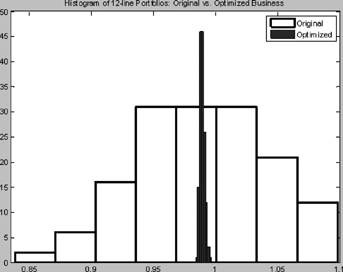
The histograms of the original and the MV+CVaR 12-Line life insurance portfolios in Figure 10 suggest that both portfolios have unimodal distributions. Similar to Figure 8 of Example 1, Figure 11 illustrates a lower risk of the MV+CVaR 12-Line portfolio than its original 12-Line counterpart: it has much narrower bounds and lower values of the right tails.
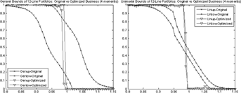
Notes: The left and right graphs show the general and unimodal bounds, respectively. In both graphs, the symbol  represents the bounds on the original portfolio. The symbol
  represents the bounds on the optimized one.
We further perform the bound analysis to compare the MV+CVaR efficient 9-Line portfolio without annuities and the MV+CVaR efficient 12-Line portfolio with annuities. As expected, Figure 12 suggests a much lower downside risk of the MV+CVaR efficient 12-Line portfolio, again, supporting the natural hedging benefits between life insurance and annuities.
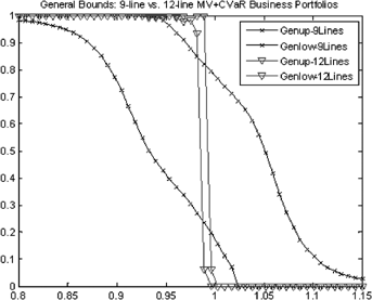
Notes: The curves with  represent the upper and lower bounds of the MV+CVaR portfolio with 9 lines of life insurance. Bounds of the optimal 12-Line mortality portfolio are shown as the
  curves.
In practice, it may be difficult for an insurer to directly accomplish an MV+CVaR optimal business composition in Portfolio (25). For example, it may not be easy for an insurer specializing in life insurance to enter the annuity business (Cox and Lin, 2007). To solve this problem, the insurer has at least two possible solutions. First, the insurer can buy or sell reinsurance to rebalance its weights in various business lines. Second, the insurer can issue or purchase mortality or longevity securities in the capital markets. The mortality-linked securities are new in the financial markets but have attracted a lot of attention from insurers, investors, pension plans, and academia (Blake and Burrows, 2001; Cowley and Cummins, 2005; Lin and Cox, 2005, 2008; Cairns, Blake, and Dowd, 2006 Cox, Lin, and Wang, 2006). As the mortality-linked security markets develop, the insurer may be able to cede or assume risk to realize the MV+CVaR efficient mortality portfolio at a low cost.
FRONTIERS OF EFFICIENT MORTALITY PORTFOLIOS
- the two- or three-dimensional representations of the Markowitz and MV+CVaR optimal portfolios;
- the two- or three-dimensional representations of the 9-Line and 12-Line optimal portfolios.
Frontiers of Markowitz and MV+CVaR Optimized Portfolios
 (26)
(26) and
and  corresponds to the 95 percent level CVaR of the original portfolio. To compare the MV+CVaR optimal portfolios with their Markowitz counterparts, we set the benchmark
  at the 95 percent CVaR of the Markowitz portfolio given the benefit payment ratio
  . This setting guarantees that the 95 percent CVaR of the MV+CVaR portfolio is no higher than that of its Markowitz counterpart. With
  specified as (26), the upper limit of 95 percent level CVaR constraint imposed on the traditional Markowitz problem changes with the risk reduction level
  . In practice, the insurer can choose a level of
  that fits its specific risk management needs. In our illustration, we choose the highest possible
  for each portfolio that keeps problem (6) feasible.
For the nine lines of business mentioned earlier, we solve (1) the traditional Markowitz portfolio problem and (2) the MV+CVaR Problem (6) with a 95 percent CVaR constraint specified by (26). We obtain a set of optimal portfolios with different benefit payment ratios. We plot the variance–mean, skewness–mean, CVaR 5percent–mean, and CVaR 95percent–mean graphs for the MV+CVaR optimal portfolios and compare them to their Markowitz counterparts. Each graph in Figure 13 is a piecewise linear interpolation based on 20 solved efficient portfolios. Note that although our MV+CVaR problem is not a typical multiple objective optimization problem, loosely speaking, it minimizes both variance and CVaR subject to a preset expected benefit payment ratio. Therefore, the efficient frontier for a MV+CVaR optimization problem is a surface in the three-dimensional space (mean, variance, CVaR). Any two-dimensional profile shown in Figure 13 is a cross-section of the three-dimensional representation with the value of the third fixed.
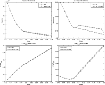
Notes: The variance–mean, skewness–mean, CVaR 5percent–mean, and CVaR 95percent–mean plots are shown in the top left, top right, bottom left, and bottom right graphs, respectively. Each graph is a piecewise linear interpolation based on 20 points. The curves with  represent the traditional Markowitz frontiers. The MV+CVaR profiles with
  specified in (26) are shown as
  curves in all graphs.
While the upper left graph of Figure 13 shows that the MV+CVaR efficient frontier somewhat deviates from the Markowitz efficient frontier in terms of the mean–variance trade-off, the MV+CVaR approach effectively decreases the skewness of relatively high variance portfolios shown in the skewness–mean profile. A lower skewness is desirable because it decreases the likelihood of obtaining higher benefit payment ratios. The CVaR95percent–mean curves in the bottom right graph demonstrates that for the same mean, the portfolios constructed from the MV+CVaR approach are able to reach a lower 95 percent CVaR, implying a lower downside mortality risk. However, the impact of adding CVaR constraint to the Markowitz model on the portfolios with low benefit payment ratio is not as significant as that on the relatively high benefit payment ratio portfolios.
It is worth noting that by adding a large percentile CVaR constraint, the MV+CVaR approach aims at reshaping the right tail of the distribution, which corresponds to high benefits. The approach has little impact on the left tail that represents low benefits. This is confirmed by the bottom left graph in Figure 13, which shows that the CVaR5percent curve of the MV+CVaR portfolios just barely differs from that of its Markowitz counterparts.
Natural Hedging for Efficient Portfolios
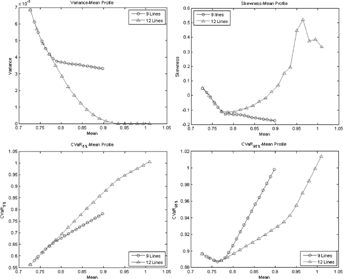
We investigate the natural hedging effect for various MV+CVaR efficient portfolios to extend our previous analysis. Given the 95 percent CVaR constraint specification (26), Figure 14 shows that the 12-Line MV+CVaR portfolios ( ) composed of both life insurance and annuity lines outperform those containing only life insurance (
 ). Given the same means, the 12-Line efficient portfolios achieve lower variance, and lower CVaR 95percent than their 9-Line counterparts. Thus, inclusion of annuities reduces the potential mortality risk (measured by variance) and downside risk (measured by CVaR 95percent) of life insurance portfolios. This provides a new evidence to support the natural hedging effects. Notice that adding annuities to a life insurance portfolio does not necessarily decrease the portfolio skewness, as shown in the upper right plot of Figure 14.
 Specified in (26)
Notes: The variance–mean, skewness–mean, CVaR 5percent–mean, and CVaR 95percent–mean plots are shown in the top left, top right, bottom left, and bottom right graphs, respectively. Each graph is a piecewise linear interpolation based on 20 points. The curves with  represent the 9-Line portfolio profiles and the
  curves stand for the profiles of the 12-Line optimized portfolios.
In our example, the improvement of the frontier by adding an annuity can be explained by the negative correlation between the annuities and the lines of life insurance, as shown in Table 9.
| Annuities | Life Insurance | 5-Year Term | 10-Year Term | Whole Life | ||||||
|---|---|---|---|---|---|---|---|---|---|---|
| (25) 1 | (35) 2 | (40) 3 | (25) 4 | (35) 5 | (40) 6 | (25) 7 | (35) 8 | (40) 9 | ||
| 10 | (65) | −0.63 | −0.64 | −0.64 | −0.86 | −0.87 | −0.87 | −0.89 | −0.92 | −0.93 |
| 11 | (70) | −0.70 | −0.71 | −0.71 | −0.91 | −0.92 | −0.92 | −0.84 | −0.87 | −0.89 |
| 12 | (75) | −0.78 | −0.79 | −0.79 | −0.96 | −0.96 | −0.96 | −0.78 | −0.81 | −0.83 |
Comparison of Markowitz and MV+CVaR Optimal Portfolios With Different values of 
A change in  in (26) alters the upper limit of 95 percent level CVaR constraint
  . The bigger the
  , the more stringent the 95 percent level CVaR constraint in (6). The MV+CVaR optimal portfolios shown in Figures 13 and 14 are determined by adding the most stringent feasible 95 percent CVaR constraints. In this section, we illustrate how the 95 percent CVaR of a MV+CVaR portfolio improves relative to its MV counterpart with various feasible risk reduction levels of
  . Specifically, we solve the MV+CVaR problem (6), subject to a 95 percent CVaR constraint with a different levels of
  , to obtain a set of optimal portfolios given a preset expected benefit payment ratios.
 . For the MV model,
  is set at 0. We show the percentage difference of 95 percent CVaR between MV and MV+CVaR optimal portfolios
 (27)
(27) specified in (26) to the traditional Markowitz problem reduces the downside risk. In general, given a specified objective benefit payment ratio
  , the percentage difference (27) increases with
  . As
. As  increases, we impose a more stringent CVaR constraint so we observe lower downside risk of MV+CVaR portfolios and bigger difference between
  and
and  .
.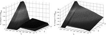

Notes: The left plot is based on 9-Line portfolios and the right one is for 12-Line portfolios. The two axes at the bottom represent the objective benefit payment ratio  and the risk reduction level
  in Equation (26), respectively.
Figure 16 shows the mean–variance–CVaR 95percent graphs for the 9-Line portfolios (left) and the 12-Line portfolios (right), respectively. In each graph, the CVaR 95percent of each MV+CVaR portfolio changes with the upper limit of the CVaR 95percent constraint  , thus forming a three-dimensional surface. As for the MV portfolios, each optimal mean and variance relationship uniquely determines a CVaR 95percent. Thus, in each graph, the mean–variance–CVaR 95percent frontier of the MV optimal portfolios is a curve represented by the dotted line. This dotted line lies above the three-dimensional surface of the MV+CVaR portfolios, suggesting the higher downside risk of the optimized MV portfolios.


Comparison of Markowitz and MV+CVaR Optimal Portfolios Using Method of Moments

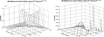
Notes: The left plot shows the probability difference of the 9-Line portfolios, and the right one is for the 12-Line portfolios. The two axes at the bottom represent the upper limit of benefit payment ratio d and the portfolio number corresponding to the 20 portfolios in Figures 13 and 14.
CONCLUSION
We applied the method of moments and portfolio optimization to mortality risk management, making two contributions to the mortality literature. First, we propose the MV+CVaR approach to manage mortality portfolio risk with a reasonable sacrifice of mean–variance efficiency. The MV+CVaR approach controls the downside risk by specifying the mean value of the benefit payment ratio above the  -level VaR to be no more than some prespecified value. This method is effective in obtaining an optimal mortality portfolio while controlling its downside risk.
Second, we applied the method of moments to mortality risk management by calculating the semiparametric upper and lower bounds on the survival function of benefit payment ratios for mortality portfolios. The bounds are used to illustrate the 100 percent confidence interval of the downside risk, which is measured by  -level VaR. We propose how to use the moments method to investigate downside risk of MV+CVaR efficient mortality portfolios. In addition, as an extension to the moments method, we derive the maximum-entropy distribution of mortality portfolios. We use the maximum-entropy approach to conduct a robustness check for the moments method because the maximum-entropy approach provides a representative distribution that is the most unbiased, given the moment information.
We illustrate our examples with up to 12 lines of business with annual observations, but these methods can be extended to more lines of business and higher frequency data. Furthermore, we would obtain more practical results by using joint forecasts of several mortality models (recognizing at least mortality for male, female, life insurance, and annuities). In addition, our results could be generalized by developing a joint model of investment and mortality risk. Such a model could be applied to a life insurer's asset liability management problem. Finally, policyholder behavior (such as surrendering the policy) is important but incorporating it will require development of new models and access to industry data. We leave these questions for future research.
APPENDIX
ESTIMATING BENEFIT PAYMENT RATIOS SUMMARIZED IN TABLE 1
 (A1)
(A1) is the time-series common risk factor that drives the mortality rates of all age cohorts. The transitory shock
  is normally distributed with zero mean. Lee and Carter model the central death rate, but usually the 1-year probability of death qx,t is very close to the central death rate. Thus, we model qx,t directly rather than model the central death rate, which would then have to be transformed to a probability.
 (A2)
(A2) (A3)
(A3)We follow a two-step procedure in Lee and Carter (1992) to estimate Model (A1). In the first step, singular value decomposition of the matrix is applied to obtain estimates for  and
and  . In the second step, the time-series common risk factor
  in year t is recalculated based on the actual number of deaths.
We assume the insurer has the same mortality experience as that of the U.S. population. The insurer uses qx,t in the U.S. male population mortality tables, observed each year from 1901 to 2005 from the Human Life Table Database and the Human Mortality Database, to estimate Model (A1). The tables for years 1901–1999 are from the Human Life Table Database and the tables for 2000–2005 are from the Human Mortality Database, published by the University of California, Berkeley and Max Planck Institute for Demographic Research.5 The age range is  for U.S. males from t = 1901 to t=2005. The parameter estimates of ax and bx are given in Table A1 and the estimated
  is shown in Figure A1.
| Age | ax | bx | Age | ax | bx | Age | ax | bx |
|---|---|---|---|---|---|---|---|---|
| 0 | −3.4280 | 0.1709 | 35 | −5.6011 | 0.1064 | 70 | −3.0273 | 0.0385 |
| 1 | −5.6995 | 0.2618 | 36 | −5.5465 | 0.1046 | 71 | −2.9482 | 0.0390 |
| 2 | −6.2021 | 0.2383 | 37 | −5.4875 | 0.1020 | 72 | −2.8689 | 0.0390 |
| 3 | −6.4978 | 0.2296 | 38 | −5.4285 | 0.0993 | 73 | −2.7897 | 0.0386 |
| 4 | −6.7050 | 0.2279 | 39 | −5.3688 | 0.0969 | 74 | −2.7116 | 0.0382 |
| 5 | −6.8580 | 0.2181 | 40 | −5.3043 | 0.0936 | 75 | −2.6329 | 0.0372 |
| 6 | −6.9871 | 0.2039 | 41 | −5.2384 | 0.0906 | 76 | −2.5543 | 0.0366 |
| 7 | −7.1118 | 0.1918 | 42 | −5.1698 | 0.0874 | 77 | −2.4736 | 0.0362 |
| 8 | −7.2246 | 0.1829 | 43 | −5.0994 | 0.0843 | 78 | −2.3915 | 0.0365 |
| 9 | −7.3294 | 0.1829 | 44 | −5.0278 | 0.0814 | 79 | −2.3026 | 0.0354 |
| 10 | −7.3991 | 0.1887 | 45 | −4.9547 | 0.0785 | 80 | −2.2265 | 0.0371 |
| 11 | −7.3766 | 0.1892 | 46 | −4.8791 | 0.0753 | 81 | −2.1464 | 0.0369 |
| 12 | −7.2279 | 0.1745 | 47 | −4.8039 | 0.0722 | 82 | −2.0703 | 0.0361 |
| 13 | −6.9995 | 0.1503 | 48 | −4.7275 | 0.0687 | 83 | −1.9986 | 0.0345 |
| 14 | −6.7722 | 0.1284 | 49 | −4.6521 | 0.0655 | 84 | −1.9298 | 0.0327 |
| 15 | −6.5673 | 0.1118 | 50 | −4.5753 | 0.0621 | 85 | −1.8621 | 0.0309 |
| 16 | −6.3911 | 0.0997 | 51 | −4.4986 | 0.0592 | 86 | −1.7936 | 0.0293 |
| 17 | −6.2538 | 0.0939 | 52 | −4.4214 | 0.0569 | 87 | −1.7243 | 0.0281 |
| 18 | −6.1434 | 0.0907 | 53 | −4.3449 | 0.0553 | 88 | −1.6541 | 0.0273 |
| 19 | −6.0631 | 0.0915 | 54 | −4.2685 | 0.0543 | 89 | −1.5838 | 0.0267 |
| 20 | −5.9922 | 0.0948 | 55 | −4.1907 | 0.0531 | 90 | −1.5141 | 0.0261 |
| 21 | −5.9248 | 0.0963 | 56 | −4.1127 | 0.0519 | 91 | −1.4449 | 0.0254 |
| 22 | −5.8865 | 0.0990 | 57 | −4.0341 | 0.0504 | 92 | −1.3773 | 0.0244 |
| 23 | −5.8748 | 0.1010 | 58 | −3.9552 | 0.0486 | 93 | −1.3120 | 0.0235 |
| 24 | −5.8818 | 0.1025 | 59 | −3.8772 | 0.0468 | 94 | −1.2491 | 0.0223 |
| 25 | −5.8969 | 0.1043 | 60 | −3.7976 | 0.0450 | 95 | −1.1920 | 0.0225 |
| 26 | −5.9044 | 0.1055 | 61 | −3.7190 | 0.0437 | 96 | −1.1357 | 0.0218 |
| 27 | −5.9035 | 0.1071 | 62 | −3.6404 | 0.0420 | 97 | −1.0807 | 0.0215 |
| 28 | −5.8871 | 0.1087 | 63 | −3.5650 | 0.0406 | 98 | −1.0282 | 0.0213 |
| 29 | −5.8555 | 0.1096 | 64 | −3.4897 | 0.0391 | 99 | −0.9796 | 0.0210 |
| 30 | −5.8209 | 0.1105 | 65 | −3.4141 | 0.0379 | 100 | −0.9305 | 0.0208 |
| 31 | −5.7849 | 0.1104 | 66 | −3.3373 | 0.0370 | 101 | −0.8823 | 0.0209 |
| 32 | −5.7455 | 0.1103 | 67 | −3.2595 | 0.0365 | 102 | −0.8352 | 0.0192 |
| 33 | −5.7013 | 0.1095 | 68 | −3.1830 | 0.0370 | 103 | −0.7830 | 0.0226 |
| 34 | −5.6540 | 0.1083 | 69 | −3.1056 | 0.0377 |
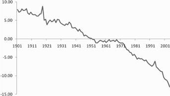
 Shown in the Vertical Axis for Year
  in the Horizontal Axis
 is assumed to follow a random walk with drift c,
 (A4)
(A4) . Based on the time series of
  where
where  , we obtain c=−0.2032 and
  .
. each year for k years. Then the common risk factor
  in year 2005+ j is calculated by adding the constant c=−0.2032 to each simulated error term e2005+ j. Given the estimated axs and bxs in Table A1, the simulated
  s, and the U.S. Treasury yield curve on December 28, 2005, we use Model ( A1 ) to calculate simulated future mortality rates

REFERENCES


